Coreflections in Algebraic Quantum Logic

Abstract

Various generalizations of Boolean algebras are being studied in algebraic quantum logic, including orthomodular lattices, orthomodular po-sets, orthoalgebras and effect algebras. This paper contains a systematic study of the structure in and between categories of such algebras. It does so via a combination of totalization (of partially defined operations) and transfer of structure via coreflections.

1 Introduction

The algebraic study of quantum logics focuses on structures like orthomodular lattices, orthomodular posets, orthoalgebras and effect algebras, see for instance [3–5, 11]. This paper takes a systematic categorical look at these algebraic structures, concentrating on (1) relations between these algebras in terms of adjunctions, and (2) categorical structure of the categories of these algebras. Typical of these algebraic structures is that they involve a partially defined sum operation that can be interpreted either as join of truth values (in orthomodular lattices/posets) or as sum of probabilities (in effect algebras).

The leading example of such a partially defined sum is addition on the (real) unit interval [0,1] of probabilities: for x,y∈[0,1] the sum is defined only if x+y≤1. Because this operation is so fundamental, the paper takes the notion of partial commutative monoid (PCM) as starting point. An effect algebra, for instance, can then be understood as an orthosupplemented PCM, in which for each element x there is a unique element x ^⊥ with .

The paper studies algebraic quantum logics via a combination of:

• totalization of the partially defined operation into a richer algebraic structure, forming a coreflection with the original (partial) structures. Such a coreflection is an adjunction where the left adjoint is a full and faithful functor;

• transfer of structure along these coreflections. It is well-known (see [1, I, Proposition 3.5.3]) that limits and colimits can be transferred from one category to another if there is a coreflection between them. Here we extend this result to include also transfer of adjunctions and of monoidal structure.

In Sect. 3 we show that effect algebras also form a reflection with test spaces (following [8, 15]), so that we have a situation:

Both the reflection and the coreflection can be used to study the categorical structure of the category of effect algebras. However, here we shall do so via the coreflection only, because this coreflection involves total operations that are easy to work with.

In particular, we obtain tensors of effect algebras via this coreflection. They are not new: they are constructed explicitly in [2, 6]. Here they simply arise from a transfer result based on coreflections. The presence of these tensors is an important advantage of effect algebras over orthomodular lattices [11]. They naturally lead to notions like ‘effect monoid’ (monoid in the category of effect algebras) and ‘effect module’ (action for such a monoid). For instance, the effects of a Hilbert space—positive operators below the identity—form an example of such an effect module, with the effect monoid [0,1] as scalars. A systematic study of these structures will appear elsewhere.

2 Partial Commutative Monoids and Effect Algebras

Before introducing the main objects of study in this paper we first recall some basic notions about commutative monoids and fix notation.

The free commutative monoid on a set A is written as $\mathcal {M}(A)$. It consists of finite multisets n ₁ a ₁+⋯+n _k a _k of elements a _i ∈A, with multiplicity n _i ∈ℕ. Such multisets may be seen as functions φ:A→ℕ with finite support, i.e. the set sup(φ)={a∈A∣φ(a)≠0} is finite. The commutative monoid structure on $\mathcal {M}(A)$ is then given pointwise by the structure in ℕ, with addition (φ+ψ)(a)=φ(a)+ψ(a) and zero element 0(a)=0. These operations can be understood as join of multisets, with 0 as empty multiset.

The mapping $A\mapsto \mathcal {M}(A)$ yields a left adjoint to the forgetful functor CMon→Sets from commutative monoids to sets. For a function f:A→B we have a homomorphism of monoids $\mathcal {M}(f): \mathcal {M}(A)\rightarrow \mathcal {M}(B)$ given by (∑ _i n _i a _i )↦(∑ _i n _i f(a _i )), or more formally, by $\mathcal {M}(f)(\varphi)(b) = \sum_{a\in f^{-1}(b)}\varphi(a)$. The unit $\iota: A\rightarrow \mathcal {M}(A)$ of the adjunction may be written as ι(a)=1a.

If M=(M,+,0) is a commutative monoid we can interpret a multiset $\varphi\in \mathcal {M}(M)$ over M as an element 〚φ〛=∑ _x∈sup(φ) φ(x)⋅x, where n⋅x is x+⋯+x, n times. In fact, this map 〚−〛 is the counit of the adjunction mentioned before. Each monoid M carries a preorder ⪯ given by: x⪯y iff y=x+z for some z∈M. In free commutative monoids $\mathcal {M}(A)$ we get a poset order φ⪯ψ iff φ(a)≤ψ(a) for all a∈A. Homomorphisms of monoids are monotone functions wrt. this order ⪯. This applies in particular to interpretations .

Definition 1

A partial commutative monoid, or PCM, is a triple consisting of a set M, an element 0∈M and a partially defined binary operation such that the three axioms below are satisfied. We let the expression ‘x⊥y’ mean ‘ is defined’, and call such elements x,y orthogonal.

• 1. x⊥y implies y⊥x and .

• 2. y⊥z and implies x⊥y and and .

• 3. 0⊥x and .

An effect algebra is a PCM with a special element 1 and an additional unary operator (−)^⊥ called the orthosupplement such that

• 1. x ^⊥ is the unique element such that .

• 2. x⊥1 implies x=0.

An orthoalgebra is an effect algebra in which x⊥x implies x=0.

In some texts (e.g. [3, 6]) it is required that 0≠1 however we allow {0} as an effect algebra since it will be the final object in the category EA. We shall call {0} the trivial effect algebra.

An obvious example of a PCM is the unit interval [0,1] of real numbers, with defined, and equal to x+y, iff this sum x+y fits in [0,1]. It even forms an effect algebra with x ^⊥=1−x.

A different class of effect algebras are the orthomodular lattices [11]. Let L=(L,∨,∧,0,1,(−)^⊥) be an orthomodular lattice. We can turn L into an effect algebra (in fact an orthoalgebra) by restricting the ∨ operator. We will let x⊥y iff x≤y ^⊥ and then set . This construction applies in particular to Boolean algebras.

Historically the notion of an orthomodular lattice is one of the first attempts at defining what a quantum logic should be. Later this notion was generalized to that of an orthomodular poset, then orthoalgebras and finally effect algebras. In this paper we focus on effect algebras but our results and techniques will also work orthoalgebras. We will not discuss orthomodular lattices and posets any further in this paper, we refer interested readers to [12, 13].

We list a few elementary properties of effect algebras.

Proposition 1

Let E be an effect algebra:

• 1. (x ^⊥)^⊥=x and 1=0^⊥.

• 2. The relation ≤, defined by x≤y iff there exists z∈E such that , is a partial order with 0 as bottom and 1 as top element.

• 3. x⊥y iff x≤y ^⊥.

• 4. x≤y iff x ^⊥≥y ^⊥.

• 5. and implies y=y′.

• 6. implies x=y=0.

Definition 2

We organize partial commutative monoids into a category PCM as follows. The objects are PCMs and homomorphisms are (total) functions from M to N such that f(0)=0, and for x,y∈M, x⊥y implies f(x)⊥f(y) and .

We also form the category EA of effect algebras. An effect algebra homomorphism is a PCM homomorphism such that f(1)=1. This condition implies that effect algebra homomorphisms preserve the orthosupplement.

Remark 1

In the beginning of this section we described the interpretation 〚∑ _i n _i x _i 〛=∑ _i n _i ⋅x _i of a multiset $(\sum_{i}n_{i}x_{i})\in \mathcal {M}(M)$ in a monoid M. In case M is a PCM, such an interpretation need not always exist. Over a PCM M we call a multiset φ an orthogonal multiset in M if the interpretation exists in M. Here we write n⋅x for the n-fold sum , assuming it exists.

We shall write $\mathcal {O}r(M)\hookrightarrow \mathcal {M}(M)$ for the subset of orthogonal multisets in M. The subset $\mathcal {O}r(M)$ is downclosed ($\varphi \preceq \psi \in \mathcal {O}r(M)$ implies $\varphi\in \mathcal {O}r(M)$), and forms a PCM itself, with the interpretations 〚−〛 forming homomorphisms of PCMs .

Notice that $1x\in \mathcal {O}r(M)$, for x∈M, so that $\bigcup_{\varphi\in \mathcal {O}r(M)}\mathsf {sup}(\varphi) = M$. For a map f:M→N in PCM, if $\varphi = (\sum_{i}n_{i}x_{i})\in \mathcal {O}r(M)$ then $\mathcal {M}(f)(\varphi) = (\sum_{i}n_{i}f(x_{i})) \in \mathcal {O}r(N)$, by definition of ‘morphism in PCM’, and:

(1)

Because the interpretation function 〚−〛 is partial for a PCM there are different forms of equality, depending on whether existence of interpretations is required or assumed.

• 1. Assuming existence leads to the following notion of ‘partial equality’; it is the one that is most frequently used for partially defined operations. We write:

  

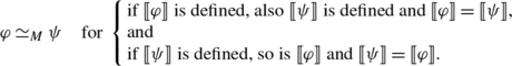  (2)

  The subscript ‘M’ in ≃ _M is sometimes omitted when M is clear from the context.

• 2. When existence is required one does not get an equivalence relation, like above, but only that what is called a partial equivalence relation (PER) $\equiv \subseteq \mathcal {M}(M)\times \mathcal {M}(M)$. It is a relation that is symmetric and transitive but not necessarily reflexive. In this case:

  

  (3)

Partial equivalence relations (PERs) are used extensively in the semantics of higher order lambda calculi, see for instance [9, 16]. In general, for a PER R⊆X×X one writes dom(R)={x∈X∣R(x,x)} for the domain of R. Notice that R(x,y) implies x,y∈dom(R). When R is restricted to dom(R)⊆X it forms an equivalence relation. Hence such a PER R gives rise to a “subquotient” of the form X↢dom(R)↠dom(R)/R.

For the PER ≡ associated in (3) with a PCM M, the subset is the domain $\mathsf {dom}(\equiv) = \{\varphi\in \mathcal {M}(M)\mid \varphi\equiv\varphi\}$ of the PER ≡. Hence ≡ is an actual equivalence relation on $\mathcal {O}r(M)$, so that one can form the quotient $\mathcal {O}r(M)/\!\equiv$.

For later use we observe the following.

Lemma 1

Partial equality $\simeq_{M}\subseteq \mathcal {M}(M)\times \mathcal {M}(M)$, for a PCM M, is an equivalence and a congruence relation.

Proof

Clearly, ≃ is an equivalence relation. Suppose φ≃φ′ and ψ≃ψ′, and assume 〚φ+ψ〛 is defined. Then both 〚φ〛 and 〚ψ〛 are defined, and . From φ≃φ′ and ψ≃ψ′ we obtain that also 〚φ′〛 and 〚ψ′〛 are defined, and 〚φ′〛=〚φ〛 and 〚ψ′〛=〚ψ〛. Hence:

so that φ+ψ≃φ′+ψ′. □

3 Tests

So-called test spaces have been introduced by Foulis and Randall [8, 15] in their reformulation of probability theory. Here we take the freedom to adapt the definition in such a way that it can also be made to work for PCMs. We will show that the constructions from [6] transforming test spaces into effect algebras and vice versa take the form of a reflection.

Definition 3

A test perspective is given by a set A together with a partial equivalence relation $\equiv_{A} \subseteq \mathcal {M}(A)\times \mathcal {M}(A)$ satisfying:

• 1. 0≡ _A 0;

• 2. φ≡ _A ψ implies $\forall {\alpha\in \mathcal {M}(A)}. \varphi+\alpha\in \mathsf {dom}(\equiv_{A}) \Rightarrow \varphi+\alpha \equiv_{A} \psi+\alpha$;

• 3. the domain dom(≡ _A )={φ∣φ≡ _A φ} covers A, in the sense that ⋃{sup(φ)∣φ∈dom(≡ _A )}=A;

We form a category TestPer with such test perspectives as objects and morphisms f:(A,≡ _A )→(B,≡ _B ) given by functions f:A→B between the underlying sets, satisfying $\varphi \equiv_{A} \psi \Rightarrow \mathcal {M}(f)(\varphi) \equiv_{B} \mathcal {M}(f)(\psi)$.

The following result shows how such structures can arise.

Lemma 2

Each PCM M yields (M,≡)∈TestPer, in a functorial manner—where $\equiv \subseteq \mathcal {M}(M)\times \mathcal {M}(M)$ is the PER introduced in Remark 1. We shall write this functor as $\mathcal {T}\hspace {-3pt}{\scriptstyle {e}}\colon \mathbf {PCM}\rightarrow \mathbf {TestPer}$. It is full and faithful.

Proof

For a PCM M we recall that the domain of the associated PER ≡ on $\mathcal {M}(M)$ is . Hence the three requirements in the definition obviously hold. For a morphism of PCMs f:M→N the resulting map $\mathcal {M}(f)\colon \mathcal {M}(M)\rightarrow \mathcal {M}(N)$ preserves these PERs ≡. Faithfulness is immediate. And for fullness we need to show that a map of test perspectives f:(M,≡)→(N,≡) is also a PCM-map f:M→N. Therefore we note that , assuming x⊥y in M, and similarly, as nullary case, 10≡0. Hence and $1f(0) = \mathcal {M}(f)(10) \equiv \mathcal {M}(f)(0) = 0$. This means that we get in N, and f(0)=〚1f(0)〛=〚0〛=0. □

In the other direction one can also turn test perspectives into PCMs. For the PCM associated with a test perspective (A,≡ _A ) we use the ad hoc notation $A{\kern -.8ex}\swarrow {\kern -2ex}\equiv _{A}$. This construction uses the downset of the domain ${\mathop {\downarrow }\mathsf {dom}(\equiv_{A})} = \{\varphi\in \mathcal {M}(A)\mid \exists {\alpha}.\varphi+\alpha\in \mathsf {dom}(\equiv_{A})\}$. It is not hard to see that φ≡ _A φ′ and φ∈ ↓dom(≡ _A ) implies φ′∈ ↓dom(≡ _A ). Thus we can define

$$\begin{array}{rcl} A{\kern -.8ex}\swarrow {\kern -2ex}\equiv _{A} & = & \big \{[\varphi]_{A}\mid \varphi\in \mathop {\downarrow }\mathsf {dom}(\equiv_{A})\big \}, \end{array}$$

where $[\varphi]_{A} \subseteq \mathcal {M}(A)$ is the equivalence class [φ] _A ={ψ∣φ≡ _A ψ}. For φ,ψ∈ ↓dom(≡ _A ) we define [φ]⊥[ψ] iff φ+ψ∈ ↓dom(≡ _A ), and in that case we take: . By the second requirement in Definition 3 this is well-defined. Clearly, $[0]_{A}\in A{\kern -.8ex}\swarrow {\kern -2ex}\equiv _{A}$ is zero element.

Proposition 2

Partial commutative monoids form a reflective category in test perspectives, in the following situation:

where the functor $\mathcal {Q}\colon \mathbf {TestPer}\rightarrow \mathbf {PCM}$ is $(A,\equiv_{A}) \mapsto A{\kern -.8ex}\swarrow {\kern -2ex}\equiv _{A}$.

Proof

For (A,≡ _A )∈TestPer and M∈PCM we have a bijective correspondence:

Given $f\colon A{\kern -.8ex}\swarrow {\kern -2ex}\equiv _{A}\rightarrow M$ we obtain $\overline{f}\colon (A,\equiv_{A}) \rightarrow (M,\equiv)$ by $\overline{f}(a) = f([1a])$. Conversely, given g:(A,≡ _A )→(M,≡) we get $\overline{g}\colon A{\kern -.8ex}\swarrow {\kern -2ex}\equiv _{A} \rightarrow M$ by . It is routine to check that these operations $\overline{(-)}$ are well-defined, and only show that they are each others inverse:

 □

Notice that the situation A=∅ is allowed in Definition 3. In that case we get $\mathcal {M}(A) = \{0\}$ and ≡={(0,0)}. Hence $A{\kern -.8ex}\swarrow {\kern -2ex}\equiv _{A}$ is the singleton PCM.

Definition 4

A test space is a test perspective (A,≡ _A ) satisfying the following additional requirement. Define the subset $\top_{A} \subseteq \mathsf {dom}(\equiv_{A}) \subseteq \mathcal {M}(A)$ of top elements as:

$$ \begin{array}{rcl} \top_{A} & = & \big \{\varphi\in \mathsf {dom}(\equiv_{A})\mid \forall {\psi\in \mathsf {dom}(\equiv_{A})}. \varphi \leq \psi \Rightarrow \varphi \equiv_{A} \psi\big \}. \end{array} $$

(4)

Then a test space should satisfy:

• 1. φ,ψ∈⊤ _A implies φ≡ _A ψ.

• 2. dom(≡ _A )= ↓⊤ _A ;

• 3. if φ≡ _A ψ and φ+α≡ _A ψ+β then α≡ _A β, for all α,β∈dom(≡ _A ).

We shall write TestSp↪TestPer for the subcategory of test spaces with morphisms f:(A,≡ _A )→(B,≡ _B ) that map ⊤ _A to ⊤ _B , in the sense that $\varphi\in\top_{A} \Rightarrow \mathcal {M}(f)(\varphi) \in\top_{B}$.

Recall from Definition 3 that 0≡ _A 0 holds in a test perspective (A,≡ _A ). This means that 0∈dom(≡ _A )= ↓⊤ _A in a test space. Hence ⊤ _A is a non-empty subset.

Note that our definition of a test space differs from the one in [6] and [3] in the fact that we take the relation ≡ _A as primitive and define ⊤ _A while in the older definition this is reversed. We chose the current approach to accommodate for PCMs where starting from ⊤ _A would make no sense.

Theorem 1

The reflection TestPer⇄PCM from Proposition 2 restricts to a reflection:

Proof

We first check that (M,≡) is a test space if M is an effect algebra. We claim that ⊤ _M as defined in (4) satisfies:

The inclusion (⊇) is easy: if 〚φ〛 exists and equals 1, and φ≤ψ in $\mathcal {M}(M)$, then 1=〚φ〛≤〚ψ〛 in M, so that 〚ψ〛=1, and thus φ≡ψ. For (⊆), assume φ∈⊤ _M but 〚φ〛≠1. Then satisfies φ≤ψ and so we get φ≡ψ because φ∈⊤ _M . But . We check the two points in the above definition.

• 1. We have , where the marked equation holds by the following argument. For the inclusion (⊆), if 〚φ〛 exists in M, then, as before φ≤φ+1(〚φ〛^⊥)∈⊤ _M . For the reverse inclusion (⊇), notice that if φ≤ψ with 〚ψ〛 existing and equal to 1, then also 〚φ〛 exists.

• 2. Suppose φ≡ψ and φ+α≡φ+β, i.e. 〚φ〛, 〚ψ〛 exist and are equal, and similarly for 〚φ+α〛 and 〚ψ+β〛. Then: . Then 〚α〛=〚β〛 because the cancellation law holds in effect algebras. Hence α≡β.

In the other direction, we prove that $A{\kern -.8ex}\swarrow {\kern -2ex}\equiv _{A}$ is an effect algebra if (A,≡) is a test space. The orthosupplement of $[\varphi]\in A{\kern -.8ex}\swarrow {\kern -2ex}\equiv _{A}$, for φ∈ ↓dom(≡ _A ), is given as follows. We use  ↓dom(≡ _A )⊆ ↓⊤ _A and write φ+α∈⊤ _A , for some $\alpha\in \mathcal {M}(A)$. Now we simply put [φ]^⊥=[α]. This is well-defined since:

• the orthosupplement does not depend on the choice of α: if both φ+α,φ+β∈⊤ _A , then φ+α≡ _A φ+β and thus α≡ _A β by requirement 3 in Definition 4; hence [α]=[β];

• the choice of representative does not matter: if φ≡ _A ψ and both φ+α∈⊤ _A and ψ+β∈⊤ _A , then φ+α≡ _A ψ+β. By requirement 2 in Definition 3 we get ψ+α≡ _A φ+α, and by transitivity ψ+α≡ _A ψ+β so that α≡ _A β and thus [φ]^⊥=[α]=[β]=[ψ]^⊥.

The top element $1\in A{\kern -.8ex}\swarrow {\kern -2ex}\equiv _{A}$ is [γ] for any γ∈⊤ _A . We still have to check that orthosupplements are unique: if . Then φ+α≡ _A γ≡ _A φ+β. But then α≡ _A β and thus [α]=[β]. Finally, if [φ]⊥1, then φ+γ∈ ↓dom(≡ _A ). But since γ∈⊤ _A and γ≤φ+γ we get γ≡ _A φ+γ. This can be reformulated as γ+0≡ _A γ+φ, and thus φ≡ _A 0, by requirement 2 in Definition 4. Thus $[\varphi] = [0] = 0 \in A{\kern -.8ex}\swarrow {\kern -2ex}\equiv _{A}$.

The adjunction $\mathcal {Q}\dashv \mathcal {T}\hspace {-3pt}{\scriptstyle {e}}$ works just like in Proposition 2. □

Test spaces have been used to construct a tensor product for effect algebras (cf. [3, 6]), however this construction is cumbersome and not very revealing. In the rest of the paper we shall pursue a different approach to constructing this tensor product making use of a coreflection rather than the reflection presented in this section.

This coreflection will embed effect algebras into structure with total operations. They are more familiar structures and easier to work with than tests, involving partial equivalence relations.

4 Coreflections

We now turn to some technical results on coreflections which will be used for various constructions with PCMs and effect algebras.

4.1 Preliminaries on Coreflections

Recall that a coreflection is an adjunction F⊣G where the left adjoint F:A→B is full and faithful, or equivalently, the unit η:id→GF is an isomorphism. It is well-known (see [1]) that in this situation A is as complete and cocomplete as B.

Theorem 2

Suppose D:J→A is a diagram in A and that l _j :L→FD _j (resp. c _j :FD _j →C) is a limit (resp. colimit) of F∘D in B then $\eta^{-1}_{D_{j}}\circ G(l_{j}):G(L)\to D_{j}$ ($G(c_{j})\circ\eta_{D_{j}}:D_{j}\to G(C)$) is a limit (colimit) of D in A.

Below we shall show that A not only inherits limits and colimits from B but also a (symmetric) monoidal structure under some mild conditions. Furthermore we can also transfer adjoints in the sense that functors with domain A will have adjoints if certain related functors with domain B have adjoints.

The following lemma proves to be central in all these results.

Lemma 3

Let F:A→B be part of a coreflection F⊣G and let B∈B. If the counit ε _B :FGB→B is a split epi then ε _B is an isomorphism.

Proof

Suppose g:B→FGB is such that ε _B ∘g=id _B then it follows that $g=\varepsilon _{B}^{-1}$ since:

where (*) follows from the fact that η _GB is an isomorphism and ε _FGB ∘F(η _GB )=id by the triangular identities. □

Since the dual notion of a coreflection is a reflection, i.e. an adjunction where the right adjoint is full and faithful and the counit an isomorphism, all results from this section can also be formulated for reflections instead.

4.2 Coreflections and Adjunctions

The situation we will be studying here is as follows. We have a coreflection (F ₁,G ₁,η ¹,ε ¹):A ₁→B ₁ and an adjunction (F ₂,G ₂,η ²,ε ²):A ₂→B ₂ as well as a map of adjunctions (H:A ₁→A ₂,K:B ₁→B ₂). This means that we have natural isomorphisms α:KF ₁→F ₂ H and β:HG ₁→G ₂ K such that the following diagrams commute for all X∈A ₁ and Y∈B ₁.

(5)

Next we suppose that K is part of an adjunction (L,K,δ,ξ) and define J:A ₂→A ₁ as J=G ₁∘L∘F ₂.

Theorem 3

In the situation described above, the functor J=G ₁ LF ₂ is left adjoint to H.

Proof

Let X∈A ₂ and define θ _X :X→HJX by $\theta_{X}=\beta_{LF_{2}X}^{-1}\circ G_{2}(\delta_{F_{2}X})\circ \eta^{2}_{X}$.

We want to show that θ _X is a universal arrow towards H. So let f:X→HY, we need to construct $\hat{f}:JX=G_{1}LF_{2}X\to Y$. To do so define f′:F ₂ X→KF ₁ Y by $f'=\alpha_{Y}^{-1}\circ F_{2}(f)$. Now using the L⊣K adjunction we can find an $\widehat{f'}:LF_{2}X\to F_{1}X$ such that $K(\widehat{f'})\circ \delta_{F_{2}X} =f'$. Now define $\hat{f} = (\eta^{1}_{Y})^{-1}\circ G_{1}(\widehat{f'})$.

(6)

We now compute:

Next we need to show that $\hat{f}$ is the only arrow with this property. Like before we need an auxiliary result. □

Lemma 4

The counit $\varepsilon ^{1}_{LF_{2}X}:F_{1}G_{1}LF_{2}X\to LF_{2}X$ is an isomorphism.

Proof (of the lemma)

We need to construct an inverse g:LF ₂ X→F ₁ G ₁ LF ₂ X using the L⊣K adjunction we can do this by constructing a map F ₂ X→KF ₁ G ₁ LF ₂ X≅F ₂ HG ₁ LF ₂ X. We can use F ₂(θ _X ) there. So define

Write $h=\varepsilon ^{1}_{LF_{2}X}\circ g :LF_{2}X\to LF_{2}X$ to show h=id we could take the transpose $\overline{h}:F_{2}X\to KLF_{2}X$ and prove $\overline{h}=\delta_{F_{2}X}$. And to show this it is enough to take $\overline{\overline{h}}:X\to G_{2}KLF_{2}X$ and show that this equals $\beta_{LF_{2}X}\circ\theta_{X}$. We have

$$\overline{\overline{h}} = G_2\bigl(K(\varepsilon ^1_{LF_2X}\circ g)\bigr) \circ G_2(\delta_{F_2X})\circ \eta^2_X $$

and compute:

Where equalities 2,6 and 8 follow from naturality, the 7th equality follows from (5) and the final equation follows from the triangular identities. Thus we have $\varepsilon ^{1}_{LF_{2}X}\circ g = \textrm {id}$. The result now follows from Lemma 3. □

Proof (Continuation of the proof of Theorem 3)

Suppose k:JX→Y is such that H(k)∘θ _X =f. We need to prove $k=\hat{f} = (\eta^{1}_{Y})^{-1}\circ G_{1}(\widehat{f'})$. To do so we define $k' = F_{1}(k)\circ (\varepsilon ^{1}_{LF_{2}X})^{-1}:LF_{2}X\to F_{1}Y$. We have

Here equality (2) follows from (5) and equalities (3) and (4) follow from naturality.

Since $\widehat{f'}$ was the unique map with this property we see $k'=\widehat{f'}$. Finally we see:

$$\begin{array}[b]{rcll} \hat{f} & = & \bigl(\eta^1_Y\bigr)^{-1}\circ G_1\bigl(\widehat{f'}\bigr) \\ & = & \bigl(\eta^1_Y\bigr)^{-1}\circ G_1F_1(k)\circ G_1\bigl( \bigl(\varepsilon ^1_{LF_2X}\bigr)^{-1}\bigr) \\ & = & k\circ \bigl(\eta^1_{G_1LF_2X}\bigr)^{-1}\circ G_1\bigl( \bigl(\varepsilon ^1_{LF_2X}\bigr)^{-1}\bigr) \qquad & \text{(naturality)} \\ & = & k. & \text{(triangular identity)} \end{array}$$

 □

We can prove a similar result for right adjoints. This will be easier to prove and involves less stringent conditions. We require (F ₁,G ₁,η ¹,ε ¹) to be an adjunction between A ₁ and B ₁ but we only require a full and faithful functor F ₂:A ₂→B ₂. Like before we suppose we have two functors H:A ₁→A ₂ and K:B ₁→B ₂ as well as a natural isomorphism α:KF ₁→F ₂ H. This time we suppose K has right adjoint R:B ₂→B ₁ and define J=G ₁∘R∘F ₂.

Theorem 4

The above functor J=G ₁ RF ₂ is right adjoint to H.

Proof

This follows from a series of natural isomorphisms as below:

 □

These results about adjunctions capture part of the results about (co)limits. If J is some index category then a category A has all (co)limits of type J iff the diagonal A→A ^J has a left or right adjoint. If F:A→B is part of a coreflection (F,G,η,ε) we can create a coreflection between A ^J and B ^J in the obvious way. Now the diagonal functors satisfy the conditions of Theorems 3 and 4 so that if B has all (co)limits of type J then so has A.

4.3 Coreflections and Monoidal Structure

In this section we will work with a coreflection (F,G,η,ε) where F:A→B. This time we will assume that B comes equipped with a (possibly symmetric) monoidal structure (⊗,I) with the standard natural coherence isomorphisms

and optionally γ:X⊗Y→Y⊗X.

Our goal is to use this monoidal structure on B to create one on A. For this we will assume that the composite functor FG:B→B is monoidal, say via (natural) maps

and that the counit ε is a monoidal natural transformation. This means ε∘ζ=id and ε∘ξ=ε⊗ε.

We now define a bifunctor ⊗^A:A×A→A by

$$ X\otimes^{{\mathbf {A}}} Y \mathrel {\mathop {:}}=G\bigl(FX\otimes^{{\mathbf {B}}} FY\bigr) $$

(7)

and also define I ^A :=G(I ^B). We omit the superscripts for these tensors and tensor units when confusion is unlikely.

We first prove a lemma

Lemma 5

The counits $\varepsilon _{I^{{\mathbf {B}}}}:F(I^{{\mathbf {A}}}) =FG(I^{{\mathbf {B}}})\to I^{{\mathbf {B}}}$ and

$$\varepsilon _{FX\otimes FY} : F\bigl(X\otimes^{{\mathbf {A}}} Y\bigr) = FG\bigl(FX\otimes^{{\mathbf {B}}} FY\bigr) \to FX\otimes^{{\mathbf {B}}} FY $$

are isomorphisms.

Proof

Because of Lemma 3 it is enough to show that these counits are split epis. Since ε is monoidal we have $\varepsilon _{I^{{\mathbf {B}}}}\circ\zeta = \textrm {id}$ and so $\varepsilon _{I^{{\mathbf {B}}}}$ is a split epi.

The candidate inverse for ε _FX⊗FY is

and we see

$$\varepsilon \circ\xi\circ \bigl(F(\eta)\otimes F(\eta)\bigr) = (\varepsilon \otimes \varepsilon )\circ \bigl(F(\eta)\otimes F(\eta)\bigr) = \textrm {id}$$

 □

As an aside we mention that in the current situation with a coreflection the induced comonad FG is not only monoidal as a functor but also as a comonad. This means that the diagonal δ=FηG:FG⇒FGFG is also a monoidal transformation. This follows because $\delta_{X} = F(\eta_{GX}) = \varepsilon _{FGX}^{-1}$ and ε is a monoidal natural transformation.

Theorem 5

In the situation sketched above:

• 1. The tensor (7) yields (symmetric) monoidal structure on the category A in such a way that the functor G:B→A is automatically monoidal, via the maps:

  

• 2. The functor F:A→B is strongly monoidal, via the isomorphism from the previous lemma:

  

• 3. If B is monoidal closed, then so is A via:

  $$B\multimap^{{\mathbf {A}}} C \mathrel {\mathop {:}}=G(FB\multimap^{{\mathbf {B}}} FC).$$

Proof

1. We can define the required isomorphisms α, ρ, λ and optionally γ in A as follows:

The coherence identities easily follow from the corresponding identities in B. The fact that G is monoidal follows from a routine computation.

2. The maps that are to make F monoidal are clearly isomorphisms. Checking the required identities is trivial.

3. This follows immediately from Theorem 4 but we also give a direct proof.

 □

5 The Categorical Structure of PCM and EA

In this section we will embed PCMs and effect algebras into algebraic structures with total operations which are easier to work with. Categorically this will take the form of a coreflection so that we can use the results from Sect. 4. The construction presented below is similar to the unigroups of Foulis, Greechie and Bennet [7]. However we use monoids instead of groups. While unigroups essentially only work for interval effect algebras our barred commutative monoids (BCMs) work for all effect algebras. Also the product of BCMs is just the Cartesian product, unlike for unigroups [7].

5.1 Totalization

Definition 5

Define a category DCM of downsets in commutative monoids as follows. Its objects consist of pairs (M,U) where M is a commutative monoid and U⊆M is a nonempty downclosed subset of M: 0∈U, and a∈U and b⪯a implies b∈U. The morphisms f:(M,U)→(N,V) consist of monoid homomorphisms f:M→N such that f(U)⊆V.

Definition 6

Define a totalization functor $\mathcal {T}\hspace {-3pt}{\scriptstyle {o}}:\mathbf {PCM}\to \mathbf {DCM}$ as follows. Let be a partial commutative monoid and put

$$\begin{array}{rcl} \mathcal {T}\hspace {-3pt}{\scriptstyle {o}}(M) & \mathrel {\mathop {:}}=& \bigl( \mathcal {M}(M)/\!\sim, \big \{[1x]_\sim\mid x\in M\big \} \bigr) \end{array}$$

where ∼ is the smallest congruence such that , for all x,y∈M with x⊥y, and $0_{\mathcal {M}(M)} \sim 1(0_{M})$. Thus, φ∼1〚φ〛, for each $\varphi\in \mathcal {O}r(M)$. Note that in $\mathcal {T}\hspace {-3pt}{\scriptstyle {o}}(M)$.

For f:M→N a homomorphism of partial commutative monoids define $\mathcal {T}\hspace {-3pt}{\scriptstyle {o}}(f)$ by $\mathcal {T}\hspace {-3pt}{\scriptstyle {o}}(f)([\sum_{i} n_{i}x_{i}]) = [\sum_{i} n_{i} f(x_{i})]$.

We will usually omit the square brackets when denoting elements of $\mathcal {T}\hspace {-3pt}{\scriptstyle {o}}(M)$, so we simply write 1x instead of [1x]_∼, and 〚φ〛 instead of 〚[φ]_∼〛. To see that $\mathcal {T}\hspace {-3pt}{\scriptstyle {o}}$ is indeed a well-defined functor we need to see that {1x∣x∈M} is actually a downset in $\mathcal {T}\hspace {-3pt}{\scriptstyle {o}}(M)$.

Lemma 6

For a PCM M we have

• (i) ∼⊆≃ where ≃ is as in Remark 1.

• (ii) If φ⪯1x in $\mathcal {T}\hspace {-3pt}{\scriptstyle {o}}(M)$, then φ∼1〚φ〛.

• (iii) {1x∣x∈M} is a downset in $\mathcal {T}\hspace {-3pt}{\scriptstyle {o}}(M)$.

Proof

For (i) recall that ≃ _M is a congruence and if x⊥y then . For (ii) suppose φ⪯1x in $\mathcal {T}\hspace {-3pt}{\scriptstyle {o}}(M)$, say via φ+ψ∼1x. Then φ+ψ≃1x, by the previous lemma. Clearly, 〚1x〛 is defined. Hence also 〚φ+ψ〛 is defined. In particular, 〚φ〛 is defined, and thus φ∼1〚φ〛.

Point (iii) follows immediately from (ii). □

To see that $\mathcal {T}\hspace {-3pt}{\scriptstyle {o}}(f)$ is well-defined note:

whenever x⊥y.

Definition 7

Define a functor $\mathcal {P}\hspace {-3pt}{\scriptstyle {a}}:\mathbf {DCM}\to \mathbf {PCM}$ by $\mathcal {P}\hspace {-3pt}{\scriptstyle {a}}(M,U) = U$, for (M,U) a monoid with downset; clearly 0∈U, and for x,y∈U we set x⊥y iff x+y∈U, and then . For a homomorphism f:(M,U)→(N,V) define $\mathcal {P}\hspace {-3pt}{\scriptstyle {a}}(f) = f|_{U}:U\to V$.

We use the fact that U is a downset in M to show that $\mathcal {P}\hspace {-3pt}{\scriptstyle {a}}(M,U)$ is a PCM. Commutativity is obvious because M is commutative. Furthermore if is defined then x+y+z∈U and because U is a downset x+y∈U and so is also defined and equal to .

Theorem 6

The totalization functor $\mathcal {T}\hspace {-3pt}{\scriptstyle {o}}:\mathbf {PCM}\to \mathbf {DCM}$ is a (full and faithful) left adjoint to $\mathcal {P}\hspace {-3pt}{\scriptstyle {a}}$. Hence we have a coreflection.

Proof

We need to construct a natural isomorphism $\eta:\textrm {id}_{\mathbf {PCM}}\to \mathcal {P}\hspace {-3pt}{\scriptstyle {a}}\mathcal {T}\hspace {-3pt}{\scriptstyle {o}}$. Let M be a PCM and define a function $\eta_{M}:M\to \mathcal {P}\hspace {-3pt}{\scriptstyle {a}}\mathcal {T}\hspace {-3pt}{\scriptstyle {o}}(M)$ by η _M (x)=1x. In $\mathcal {T}\hspace {-3pt}{\scriptstyle {o}}(M)$ we have 10 _M =0 and , for x⊥y, so that η _M is a PCM homomorphism. Using Lemma 6 part (i) we see that if 1x=1y in $\mathcal {T}\hspace {-3pt}{\scriptstyle {o}}(M)$ then 1x≃1y so that x=〚1x〛=〚1y〛=y, making η _M injective. Since $\mathcal {P}\hspace {-3pt}{\scriptstyle {a}}\mathcal {T}\hspace {-3pt}{\scriptstyle {o}}(M) = \{1x\mid x\in M\}$ it is clear that η _M is surjective.

We still need to check that $\eta_{M}^{-1}$ is a PCM homomorphism. Of course whenever 1x⊥1y in $\mathcal {P}\hspace {-3pt}{\scriptstyle {a}}\mathcal {T}\hspace {-3pt}{\scriptstyle {o}}(M)$ then 1x+1y=1z for some z. Again by Lemma 6 we get x⊥y and . So we see that η _M is an isomorphism. It is clearly natural.

To see that η _M is universal note that when we have a PCM homomorphism $f:M\to \mathcal {P}\hspace {-3pt}{\scriptstyle {a}}(N,V)$, for some monoid with downset (N,V), then f is a function from M to N. We can extend f to a monoid homomorphism $\overline{f}$ from the free monoid $\mathcal {M}(M)$ to N, by $\overline{f}(\sum_{i}n_{i}x_{i}) = \sum_{i}n_{i}f(x_{i})$. Now we see $\overline{f}(10_{M}) = f(0_{M}) = 0_{N} = \overline{f}(0)$ and:

where the third equality follows from the fact that f is a PCM homomorphism. As a result $\overline{f}$ factors through $\mathcal {T}\hspace {-3pt}{\scriptstyle {o}}(M)$. This factorization gives us a monoid homomorphism $g:\mathcal {T}\hspace {-3pt}{\scriptstyle {o}}(M)\to N$ such that g(1x)=f(x). Since f(x)∈V by assumption, we get g is a morphism $\mathcal {T}\hspace {-3pt}{\scriptstyle {o}}(M) \rightarrow (N,V)$ in DCM, with $f=\mathcal {P}\hspace {-3pt}{\scriptstyle {a}}(g)\mathrel {\circ }\eta_{M}$. It is clear that this g is unique. □

We now turn to a similar construction for effect algebras.

Definition 8

A barred commutative monoid (or BCM) (M,+,0,u) is a commutative monoid (M,+,0) that is positive i.e. a+b=0 implies a=b=0 together with an element u∈M called the unit such that a+b=a+c=u implies b=c.

The name barred commutative monoid comes from the fact that the unit forms a bar, below which certain properties must hold. However beyond this bar those properties need not hold, for example the cancellation law holds for elements below the bar but it generally need not hold for arbitrary elements in a barred commutative monoid.

Definition 9

We form the category BCM of barred commutative monoids as follows. Let the objects be the BCMs (M,+,0,u) and let the homomorphisms f:(M,+,0,u)→(M′,+,0,u′) be monoid homomorphisms M→M′ such that f(u)=u′.

Definition 10

If E is some BCM and x∈E is such that x⪯u then we call the unique y with x+y=u the complement of x and write y=x ^⊥.

We view the category BCM as a (non full) subcategory of DCM by taking the unit interval {a∈M∣a⪯u} as the required downset. Similarly we view EA as a subcategory of PCM.

Proposition 3

We can restrict the functors $\mathcal {T}\hspace {-3pt}{\scriptstyle {o}}$ and $\mathcal {P}\hspace {-3pt}{\scriptstyle {a}}$ to EA and BCM. This remains a coreflection.

Proof

We need to check that whenever E is an effect algebra then $\mathcal {T}\hspace {-3pt}{\scriptstyle {o}}(E)$ is a BCM. We let 11 _E be the unit of $\mathcal {T}\hspace {-3pt}{\scriptstyle {o}}(E)$. Using Lemma 6 we see that the unit interval of $\mathcal {T}\hspace {-3pt}{\scriptstyle {o}}(E)$ is {1x∣x∈E}.

To see that $\mathcal {T}\hspace {-3pt}{\scriptstyle {o}}(E)$ is positive let $a,b\in \mathcal {T}\hspace {-3pt}{\scriptstyle {o}}(E)$ with a+b=0. Clearly a+b⪯11 _E so also a,b⪯11 _E . So there are x,y∈E such that a=1x and b=1y. Now we get 1x+1y=0=10 _E so x⊥y and . Because E is an effect algebra we see x=y=0 and so a=b=0.

Now suppose a+b=a+c=11 _E , like before there are x,y,z∈E such that a=1x, b=1y and c=1z. Now using Lemma 6 again we see that and so y=z and therefore b=c.

We also need to check that when F is a BCM then $\mathcal {P}\hspace {-3pt}{\scriptstyle {a}}(F)$ is an effect algebra. But because F is positive we see that $\mathcal {P}\hspace {-3pt}{\scriptstyle {a}}(F)$ is positive and because a+b=u=a+c in F implies c=b we see that complements in $\mathcal {P}\hspace {-3pt}{\scriptstyle {a}}(F)$ are unique.

It is also clear that $\mathcal {P}\hspace {-3pt}{\scriptstyle {a}}$ maps BCM homomorphisms to effect algebra homomorphisms and similarly for $\mathcal {T}\hspace {-3pt}{\scriptstyle {o}}$.

Finally note that $\eta_{E}:E\to \mathcal {P}\hspace {-3pt}{\scriptstyle {a}}\mathcal {T}\hspace {-3pt}{\scriptstyle {o}}(E)$ is in fact an effect algebra homomorphism since it maps 1 _E to 11 _E which is the unit of $\mathcal {P}\hspace {-3pt}{\scriptstyle {a}}\mathcal {T}\hspace {-3pt}{\scriptstyle {o}}(E)$. □

Example 1

Here are a few examples of what the totalization of an effect algebra looks like.

• $\mathcal {T}\hspace {-3pt}{\scriptstyle {o}}([0,1])\cong \mathbb{R}_{\geq 0}$

• $\mathcal {T}\hspace {-3pt}{\scriptstyle {o}}(\mathcal{P}(X)) \cong \mathbb{N}^{X}$.

We can do something similar for orthoalgebras. If M∈BCM then $\mathcal {P}\hspace {-3pt}{\scriptstyle {a}}(M)$ is an orthoalgebra iff a+a⪯u implies a=0. We can then take the full subcategory of such objects and in this way we obtain a coreflection for orthoalgebras. If one does this then all the results below can also be obtained for orthoalgebras with minor changes to the proofs.

Remark 2

We have introduced the notion of a barred commutative monoid purely for the purpose of creating the coreflection between EA and BCM. However frequently the totalization of an effect algebra has more structure. For example consider the effects $\mathcal {E}{\kern -.5ex}f(\mathcal{H})$ of a Hilbert space $\mathcal{H}$, recall that $\mathcal {E}{\kern -.5ex}f(\mathcal{H})$ consists of the positive operators on $\mathcal{H}$ that are less than the unit. Then $\mathcal {T}\hspace {-3pt}{\scriptstyle {o}}(\mathcal {E}{\kern -.5ex}f(\mathcal{H}))$ is isomorphic to the collection of all positive operators on $\mathcal{H}$.

5.2 Limits and Colimits

The categories PCM, EA, DCM and BCM will all turn out to be both complete and cocomplete. Products, coproducts and equalizers can be described directly in all categories. But coequalizers in PCM and EA are a different story. However thanks to Theorem 2 it suffices to describe them in DCM and BCM. We start with limits and colimits in DCM. They are basically obtained as for commutative monoids.

Proposition 4

Let I be some set and let {(M _i ,U _i )∣i∈I} be a family of monoids with downsets, indexed by I.

• (a) The product of this family in DCM is:

  $$\textstyle \bigl( \prod_{i\in I}M_i, \big \{\phi\in \prod_{i\in I} M_i\mid \forall {i\in I}.\phi(i)\in U_i\big \} \bigr), $$

  where ∏ _i∈I M _i is the product of monoids. It consists of functions ϕ:I→⨆ _i∈I M _i with ϕ(i)∈M _i for all i, with the operation defined pointwise. Here ⨆ denotes the disjoint union of the underlying sets.

• (b) The coproduct is given by

  $$\textstyle \bigl(\coprod_{i\in I}M_i, \big \{\phi\in \coprod_{i\in I} M_i\mid \exists {i\in I}.\phi(i)\in U_i\ \textit{and}\ \forall {j}.i\neq j\Rightarrow \phi(j)=0\big \} \bigr), $$

  where ∐ _i∈I M _i is the monoid coproduct. It consists of functions ϕ:I→⨆ _i∈I M _i with ϕ(i)∈M _i and {i∈I∣ϕ(i)≠0} is finite.

Next, let f,g:(M,U)→(N.V) be two arrows in DCM.

• (c) The equalizer of f and g is (E,W) where E={m∈M∣f(m)=g(m)} and W=E∩U.

• (d) The coequalizer of f and g is (N/∼,{[v]∣v∈V}) where ∼ is the smallest monoid congruence such that f(m)∼g(m).

Since DCM has all products and coproducts as well as equalizers and coequalizers we see that DCM is both complete and cocomplete.

Proposition 5

Let I be a set and let {M _i ∣i∈I} be a family of PCMs.

• (a) The product of this family is given by the Cartesian product ∏ _i∈I M _i .

• (b) The coproduct is given by the disjoint union (⨆ _i∈I M _i ∖{0})∪{0} with all the 0 elements identified.

Proof

• (a) The operation on the product is defined pointwise. If ϕ,ψ∈∏ _i∈I M _i then ϕ⊥ψ iff ϕ(i)⊥ψ(i) for all i∈I and then . The projections are just the set-theoretic ones. They are easily seen to be PCM homomorphisms.

• (b) The operation on the coproduct is defined as follows

  

The obvious inclusions are PCM homomorphism and turn this construction into the coproduct. □

Proposition 6

Let f,g:M→N be two PCM homomorphisms.

• (a) The equalizer of f and g is E={m∈M∣f(m)=g(m)}.

• (b) The coequalizer of f and g is $\mathcal {P}\hspace {-3pt}{\scriptstyle {a}}(h)\mathrel {\circ }\eta_{N}$ where $h:\mathcal {T}\hspace {-3pt}{\scriptstyle {o}}(N)\to \mathcal {T}\hspace {-3pt}{\scriptstyle {o}}(N)/\!\!\sim$ is the coequalizer of $\mathcal {T}\hspace {-3pt}{\scriptstyle {o}}(f)$ and $\mathcal {T}\hspace {-3pt}{\scriptstyle {o}}(g)$ (cf. Theorem 2).

We now turn to EA and BCM. Products and equalizers in EA and BCM are constructed in the same way as in PCM and DCM. The products are just the Cartesian products with pointwise operations and the equalizers are just the set-theoretic ones.

Before tackling colimits we first study congruences on BCMs and see what consequences this has for effect algebras.

Definition 11

A congruence ∼ on a BCM E is an equivalence relation such that the following conditions hold:

• (i) a ₁∼a ₂ and b ₁∼b ₂ implies a ₁+b ₁∼a ₂+b ₂;

• (ii) a+b∼0 implies a∼0 and b∼0;

• (iii) a+b∼u and a+c∼u implies b∼c.

We will denote the set of all congruences on E with $\operatorname{Cong}(E)$.

Definition 12

If M is some monoid and u∈M is an element and ∼ is a monoid congruence on M then we call ∼ a bar congruence with respect to u if it satisfies conditions (ii) and (iii) from Definition 11.

Proposition 7

• (a) If (E,+,0,u) is a BCM and ∼ is a congruence on E then E/∼ is a BCM with unit [u]_∼. There exists a canonical surjective homomorphism π:E→E/∼ that sends x to [x]_∼.

• (b) When M is a monoid and ∼ is a bar congruence with respect to u then M/∼ is an BCM with unit [u]_∼.

Proof

(a): Addition on E/∼ is defined by [a]+[b]=[a+b] this is well-defined thanks to condition (i). Condition (ii) makes sure that E/∼ is positive since if [a]+[b]=0 then a+b∼0 and so a∼0 and b∼0. To show that [u] is a cancellative unit note that [a]+[b]=[u]=[a]+[c] implies a+b∼u∼a+c and so b∼c by condition (iii). The fact that π is a homomorphism is obvious as is its surjectivity.

(b): The proof is analogous to that of (a). □

Proposition 8

If M is a monoid and E is a BCM and f:M→E is a monoid homomorphism then if c∈M is such that f(c)=u then ker(f)={(a,b)∣f(a)=f(b)} is a bar congruence with respect to c.

The main advantage of BCM over EA (and of DCM over PCM) is that the intersection of congruences is again a congruence. So it makes sense to talk about the smallest congruence containing a given relation.

Example 2

Dividing out congruences in BCM gives rise to some epis in EA that do not occur by dividing out some equivalence on an effect algebra. For example, consider E=MO(4)={0,a,b,c,d,a ^⊥,b ^⊥,c ^⊥,d ^⊥,1} and F:=℘({a,b,c,d}) both viewed as effect algebras.

There is an effect algebra homomorphism from E to F that maps x to {x} for x∈{a,b,c,d}. It is readily seen to be an epi in EA. However F has 16 elements whereas E has 10 so clearly F does not arise by dividing out some congruence on E. However consider the congruence ∼ on $\mathcal {T}\hspace {-3pt}{\scriptstyle {o}}(E)$ generated by 1a+1b+1c+1d∼11 _E then we see that $\mathcal {T}\hspace {-3pt}{\scriptstyle {o}}(F)\cong \mathcal {T}\hspace {-3pt}{\scriptstyle {o}}(E)/\!\!\sim$.

We now move on to the construction of coproducts and coequalizers in BCM and EA.

Proposition 9

Let I be a nonempty set and let (E _i ) _i∈I be a collection of barred commutative monoids. Let C:=∐ _i∈I E _i be the monoid coproduct of the E _i and let κ _i :E _i →C be the inclusions. Choose some i∈I and let ∼ be the smallest bar congruence with respect to κ _i (u) such that for all j∈I we have κ _j (u)∼κ _i (u). The coproduct of the E _i in BCM is given by C/∼. The choice of i does not make a difference.

Proof

Let F∈BCM and let f _i :E _i →F be a collection of homomorphisms. Since each f _i is a monoid homomorphism we get a monoid homomorphism f:C→F such that f _i =f∘κ _i . By Lemma 8 the kernel of f is a bar congruence with respect to κ _i (u) for any i. As a result ∼⊆ker(f) and so f factors uniquely through C/∼. □

The empty coproduct also exists and is the initial object (ℕ,+,0,1).

Proposition 10

Let I be a set and let (E _i ) _i∈I be a collection of non-trivial effect algebras. Their coproduct is given by their disjoint union with zeros and units identified.

$$\textstyle\coprod_{i\in I} E_i = \bigl(\bigsqcup_{i\in I}E_i\setminus \{0,1\}\bigr) \cup \{0,1\} $$

The operations are defined like for PCMs.

If one of the E _i was trivial then the coproduct is also trivial due to the fact that the trivial effect algebra is a strict final object.

Proposition 11

(a) If f,g:E→F are two BCM maps then their coequalizer is given by π:F→F/∼ where ∼ is the smallest congruence containing {(f(a),g(a))∣a∈E}.

(b) For two effect algebra maps f,g:E→F their coequalizer is given by $\mathcal {T}\hspace {-3pt}{\scriptstyle {o}}(h)\mathrel {\circ }\eta_{E}$ where $h:\mathcal {T}\hspace {-3pt}{\scriptstyle {o}}(F)\to \mathcal {T}\hspace {-3pt}{\scriptstyle {o}}(F)/\!\!\sim$ is the coequalizer of $\mathcal {T}\hspace {-3pt}{\scriptstyle {o}}(f)$ and $\mathcal {T}\hspace {-3pt}{\scriptstyle {o}}(g)$ in BCM.

Since creating the coequalizer of f,g in EA involves dividing out a congruence BCM, it can happen that the coequalizer of two morphisms is not surjective. An example: let E=℘({a,x,b})+℘({c,y,d}) and F=℘({a,b,c,d}) and let 2²={0,p,p ^⊥,1}. Below are pictures of 2² and E, a picture of F can be found on page 22.

There are two maps f,g:2²→E such that f(p)={a,b} and g(p)=y. There is also a map h:E→F such that h({z})={z} for all z∈{a,b,c,d}, h({x})={c,d} and h({y})={a,b}. Note that F has 16 elements while E only has 14.

To see that h is the coequalizer of f and g let k:E→G be an effect algebra homomorphism such that k∘f=k∘g. We need to construct k′:F→G such that k=k′∘h. k′ is easily defined on the atoms and coatoms of F and also on {a,b} and {c,d}. We have no choice to send {a,c} to but we need to know this is defined. We have

so by the associativity axiom k(a)⊥k(c). A similar argument works for the remaining elements of F.

5.3 Tensor Products

Definition 13

Let M,N,L be partial commutative monoids. A bimorphism (of PCMs) f is a function f:M×N→L such that

for all m,m ₁,m ₂∈M and n,n ₁,n ₂∈N. An effect algebra bimorphism is a PCM bimorphism such that f(1,1)=1.

Let (M,U),(N,V),(L,W) be commutative monoids with downsets. A bimorphism (of monoids with downsets) f is a function f:M×N→L such that

for all m,m ₁,m ₂∈M, n,n ₁,n ₂∈N, u∈U and v∈V. A bimorphism of barred commutative monoids is a bimorphism of monoids with downsets such that f(u,u)=u.

We recall the usual definition of tensor products in terms of bimorphisms.

Definition 14

Let M and N be PCMs (or effect algebras, monoids with downsets or BCMs). A tensor product of M and N is a pair (T,t) consisting of a PCM (effect algebra, …) T and a universal bimorphism t:M×N→T such that for every bimorphism f:M×N→L there is a unique homomorphism g:T→L such that f=g∘t.

Of course the tensor product is unique up to isomorphism should it exist. We will now construct the tensor product for all four categories DCM, PCM, BCM, EA.

We will write ⊠ for the tensor product in the category CMon of commutative monoids, with the universal bimorphism M×N→M⊠N given by (m,n)↦m⊠n.

Definition 15

Let (M,U),(N,V)∈DCM, define:

$$(M,U)\otimes (N,V) = \bigl(M\boxtimes N,\mathop {\downarrow }\{u\boxtimes v\mid u\in U, v\in V\}\bigr) $$

Theorem 7

Let (M,U),(N,V)∈DCM, (M,U)⊗(N,U) together with the map χ:(m,n)↦m⊠n forms the tensor product of (M,U) and (N,V).

Proof

The map χ is readily seen to be a bimorphism. If (L,W)∈DCM and ϕ:M×N→L is a bimorphism then ϕ is also a monoid bimorphism. Therefore ϕ factors through M⊠N say by ψ, so ϕ=ψ∘χ. We still need to check that ψ is a morphism in DCM. It suffices to show that ψ(u⊠v)∈W for u∈U and v∈V. But this is clear because ϕ(u,v)∈W. □

The category DCM is symmetric monoidal. The tensor unit is (ℕ,{0,1}) and the coherence isomorphisms are inherited from CMon. We want to apply Theorem 5 to create a monoidal structure on PCM. So we must show that $\mathcal {T}\hspace {-3pt}{\scriptstyle {o}}\mathrel {\circ }\mathcal {P}\hspace {-3pt}{\scriptstyle {a}}$ is a monoidal functor.

Since $\varepsilon :\mathcal {T}\hspace {-3pt}{\scriptstyle {o}}\mathcal {P}\hspace {-3pt}{\scriptstyle {a}}(\mathbb {N},\{0,1\})\to(\mathbb {N},\{0,1\})$ is an isomorphism we set ζ=ε ⁻¹. To construct $\xi:\mathcal {T}\hspace {-3pt}{\scriptstyle {o}}\mathcal {P}\hspace {-3pt}{\scriptstyle {a}}(M,U)\otimes \mathcal {T}\hspace {-3pt}{\scriptstyle {o}}\mathcal {P}\hspace {-3pt}{\scriptstyle {a}}(N,V)\to \mathcal {T}\hspace {-3pt}{\scriptstyle {o}}\mathcal {P}\hspace {-3pt}{\scriptstyle {a}}( (M,U)\otimes (N,V))$ we use the bimorphism

It is easy to check that this is natural and that ε is a monoidal natural transformation.

Thus we get a symmetric monoidal structure on PCM given by $M\otimes N=\mathcal {P}\hspace {-3pt}{\scriptstyle {a}}(\mathcal {T}\hspace {-3pt}{\scriptstyle {o}}(M)\otimes \mathcal {T}\hspace {-3pt}{\scriptstyle {o}}(N))$. This construction is in fact a tensor product in the sense of Definition 14.

Theorem 8

If M and N are PCMs then $\mathcal {P}\hspace {-3pt}{\scriptstyle {a}}(\mathcal {T}\hspace {-3pt}{\scriptstyle {o}}(M)\otimes \mathcal {T}\hspace {-3pt}{\scriptstyle {o}}(N))$ together with the map (x,y)↦1x⊠1y is the tensor product of M and N.

Proof

Let ϕ:M×N→L be a bimorphism. We can extend ϕ to a bimorphism $\overline{\phi}:\mathcal {T}\hspace {-3pt}{\scriptstyle {o}}(M)\times \mathcal {T}\hspace {-3pt}{\scriptstyle {o}}(N)\to \mathcal {T}\hspace {-3pt}{\scriptstyle {o}}(L)$ as follows.

$$\overline{\phi}\Biggl(\sum_{i=n}^k n_ix_i,\sum_{j=1}^l m_jy_j\Biggr) = \sum_{i=1}^k\sum_{j=1}^l n_im_j\phi(x_i,y_j). $$

This is well-defined because ϕ is a bimorphism. It is clear from the definition that $\overline{\phi}$ is again a bimorphism. So we get a homomorphism $\psi:\mathcal {T}\hspace {-3pt}{\scriptstyle {o}}(M)\otimes \mathcal {T}\hspace {-3pt}{\scriptstyle {o}}(N)\to \mathcal {T}\hspace {-3pt}{\scriptstyle {o}}(L)$ such that $\psi(m\otimes n) = \overline{\phi}(m,n)$ for all $m\in \mathcal {T}\hspace {-3pt}{\scriptstyle {o}}(M)$ and $n\in \mathcal {T}\hspace {-3pt}{\scriptstyle {o}}(M)$. In particular $\psi(1x\boxtimes 1y) =\overline{\phi}(1x,1y)= 1\phi(x,y)$ for all x∈M and y∈N.

So define $\overline{\psi}:\mathcal {P}\hspace {-3pt}{\scriptstyle {a}}(\mathcal {T}\hspace {-3pt}{\scriptstyle {o}}(M)\otimes \mathcal {T}\hspace {-3pt}{\scriptstyle {o}}(N))\to L$ as $\overline{\psi} = \eta_{L}^{-1}\mathrel {\circ }\mathcal {P}\hspace {-3pt}{\scriptstyle {a}}(\psi)$ and then we see that $\overline{\psi}(1x\boxtimes 1y)=\phi(x,y)$. This factorization is clearly unique. □

Definition 16

Let E,F be two barred commutative monoids. Define E⊗F :=(E⊠F)/∼, where ⊠ is the commutative monoid tensor product and ∼ is the smallest bar congruence with respect to u⊠u. We will denote the ∼ equivalence class of e⊠f by e⊗f.

Theorem 9

Let E,F be BCMs, E⊗F together with the map χ:(e,f)↦e⊗f forms the tensor product of E and F.

Proof

The map χ:(e,f)↦e⊗f is a bimorphism thanks to the defining relations of ∼. To see that it is universal let ϕ:E×F→D be a bimorphism. Define ψ:E⊗F→D by ψ(e⊗f)=ϕ(e,f). To see that this is well defined note that ϕ is also a monoid bimorphism therefore we get a monoid homomorphism $\overline{\phi}:E\boxtimes F\to D$. But the kernel of this map is a bar congruence with respect to u⊠u so $\overline{\phi}$ factors through E⊗F.

 □

Like DCM the category BCM is also symmetric monoidal and the functor $\mathcal {T}\hspace {-3pt}{\scriptstyle {o}}\mathcal {P}\hspace {-3pt}{\scriptstyle {a}}$ is monoidal with (ℕ,1) as the tensor unit. So EA is also symmetric monoidal and just like before this monoidal structure on EA is in fact a tensor.

Theorem 10

If E and F are effect algebras then $\mathcal {P}\hspace {-3pt}{\scriptstyle {a}}(\mathcal {T}\hspace {-3pt}{\scriptstyle {o}}(E)\otimes \mathcal {T}\hspace {-3pt}{\scriptstyle {o}}(F))$ together with the map (x,y)↦1x⊗1y is the tensor product of E and F. The tensor unit is the two element effect algebra {0,1}.

Proof

The proof is analogous to that of Theorem 8. □

The categories DCM and PCM are in fact closed symmetric monoidal categories as we will see in a moment. BCM and EA are not. One cannot give $\operatorname{Hom}(E,F)$ an effect algebra structure for arbitrary effect algebras E and F. If one tries to define and ⊥ pointwise, the following problem pops up f ^⊥(1)=f(1^⊥)=f(0)=0. This problem does not occur in PCM and DCM.

Definition 17

Let (M,U),(N,V)∈DCM define an exponent:

$$(M,U)\multimap (N,V) \mathrel {\mathop {:}}=\bigl(\operatorname{Hom}_{\mathbf {CMon}}(M,N),\operatorname{Hom}_{\mathbf {DCM}}\bigl((M,U),(N,V)\bigr)\bigr) $$

This exponent is again a commutative monoid with a downset in the obvious way.

For M,N∈PCM define $M\multimap N \mathrel {\mathop {:}}=\operatorname{Hom}_{\mathbf {PCM}}(M,N)$, where the PCM structure on M⊸N is as follows. For f,g:M→N we define by . Of course is only defined when f(m)⊥g(m) for all m∈M.

We view ⊸ as a bifunctor in the usual way.

Theorem 11

For M∈PCM (or DCM) the functor M⊸(−) is a right adjoint to the functor (−)⊗M.

Since EA is monoidal we can talk about monoids in EA. The real unit interval [0,1] is such a monoid, since multiplication is a bimorphism we can view it as a morphism [0,1]⊗[0,1]→[0,1]. A state on an effect algebra E is essentially just a homomorphism from E to [0,1]. If E and F are two effect algebras equipped with a state then their tensor product also admits a state, and therefore is non trivial (see [3]).

The role of [0,1] can be played by any monoid

in EA that is non trivial. For two effect algebras E,F with morphisms s:E→M and t:F→M, the tensor product E⊗F is non trivial if M is since m∘s⊗t is a morphism E⊗F→M.

We can now also describe monoid actions in EA. They consist of a map a:M⊗E→E that commutes appropriately with the monoid maps. For the interval [0,1] such monoid actions (or effect modules) are exactly the convex effect algebras from [14].

If M is an effect module then, since $\mathcal {T}\hspace {-3pt}{\scriptstyle {o}}([0,1])\cong\mathbb{R}_{\geq 0}$, $\mathcal {T}\hspace {-3pt}{\scriptstyle {o}}(M)$ carries a ℝ_≥0 action. In fact it can be shown that $\mathcal {T}\hspace {-3pt}{\scriptstyle {o}}(M)$ carries the structure of an abstract positive cone. In [10] we have use this and other results from this paper in order to obtain a duality for effect modules.

References

Borceux, F.: Handbook of Categorical Algebra. Encyclopedia of Mathematics, vols. 50, 51, 52. Cambridge University Press, Cambridge (1994)
Dvurečenskij, A.: Tensor product of difference posets. Trans. Am. Math. Soc. 347(3), 1043–1057 (1995)
Dvurečenskij, A., Pulmannová, S.: New Trends in Quantum Structures. Kluwer Academic, Dordrecht (2000)
Engesser, K., Gabbay, D.M., Lehmann, D. (eds.): Handbook of Quantum Logic and Quantum Structures. Elsevier, Amsterdam (2007)
Foulis, D.J., Bennett, M.K.: Effect algebras and unsharp quantum logics. Found. Phys. 24(10), 1331–1352 (1994)
Foulis, D.J., Bennett, M.K.: Tensor products of orthoalgebras. Order 10(3), 271–282 (1994)
Foulis, D.J., Greechie, R.J., Bennett, M.K.: The transition to unigroups. Int. J. Theor. Phys. 37(1), 45–63 (1998)
Foulis, D.J.: C. Randall. Operational statistics I: basic concepts. J. Math. Phys. 13, 1667–1675 (1972)
Jacobs, B.: Categorical Logic and Type Theory. North Holland, Amsterdam (1999)
Jacobs, B., Mandemaker, J.: The expectation monad. In: EPTCS Proceedings of Quantum Physics and Logic (2011) (to appear)
Kalmbach, G.: Orthomodular Lattices. Academic Press, London (1983)
Pták, P.: Categories of orthomodular posets. Math. Slovaca 35, 59–65 (1985)
Pták, P., Pulmannová, S.: Orthomodular Structures as Quantum Logics. Kluwer Academic, Dordrecht, Boston, London (1991)
Pulmannová, S., Gudder, S.: Representation theorem for convex effect algebras. Comment. Math. Univ. Carol. 39(4), 645–659 (1998). Available from http://dml.cz/dmlcz/119041
Randall, C., Foulis, D.J.: Operational statistics II: manuals of operations and their logics. J. Math. Phys. 14, 1472–1480 (1973)
Streicher, Th.: Semantics of type theory. Correctness, completeness and independence results. In: Progress in Theor. Comp. Sci. Birkhäuser, Boston (1991)
Open Access
This article is distributed under the terms of the Creative Commons Attribution License which permits any use, distribution, and reproduction in any medium, provided the original author(s) and the source are credited.
Author information
Authors and Affiliations
Corresponding author
Rights and permissions
Open Access This article is distributed under the terms of the Creative Commons Attribution 2.0 International License (https://creativecommons.org/licenses/by/2.0), which permits unrestricted use, distribution, and reproduction in any medium, provided the original work is properly cited.
About this article
Cite this article
Jacobs, B., Mandemaker, J. Coreflections in Algebraic Quantum Logic. Found Phys 42, 932–958 (2012). https://doi.org/10.1007/s10701-012-9654-8
Received:
Accepted:
Published:
Issue Date:
DOI: https://doi.org/10.1007/s10701-012-9654-8