Constant yield displacement procedure for seismic evaluation of existing structures

Abstract

The starting point of the proposed procedure for seismic evaluation of existing structures is that the yield displacement of a structure in flexure is constant and that it depends only on the yield strain of the yielding material and the geometrical characteristics of the structure, not on the yield strength of that structure. The fundamental vibration period of the structure is, thus the dependent variable derived from the estimated yield strength and yield displacement of the structure. To facilitate an evaluation of the maximum inelastic deformation of an existing structure using a corresponding single-degree-of-freedom system approach, a new relation between the yield strength (defined using a new yield strength reduction factor) and the displacement ductility demand of a corresponding single-degree-of-freedom system is proposed. This relation is consistent with the constant yield displacement assumption and characterizes the relevant properties of the structure using the yield strain of its yield material, its aspect ratio and its size. The proposed Constant-Yield-Displacement-Evaluation (CYDE) procedure for seismic evaluation of existing structures has four steps. Given an existing structure, its seismic hazard environment, and an estimate of its strength, the CYDE procedure estimates the displacement ductility demand, i.e. the maximum inelastic displacement, the structure may experience at the examined seismic hazard levels. The proposed CYDE evaluation procedure is similar to the current constant-period procedures, but provides a more realistic estimate of the displacement ductility demand for stiff structures, enabling a more accurate seismic assessment of numerous existing structures.

1 Introduction

Evaluation of existing structures to examine their seismic behavior and assess their performance and safety at various seismic hazard levels is a difficult task. Structural characteristics and seismic hazard are the main sources of uncertainty in a seismic evaluation procedure due to the aging of construction material, cyclic deterioration in strength and stiffness characteristics considering experienced ground motions and the seismicity of the region to generate an expected event. Engineers’ tasks are often further compounded by the need to undertake economically justifiable retrofit actions based on the outcome of the conducted seismic evaluation.

Modern code provisions (e.g. the ASCE 31-41 family (ASCE 31-03 2003; ASCE 41-06 2006; ASCE 41-13 2013; ASCE 41-17 2017) and Eurocode 8 Part 3 (2004) address the complexity of existing building seismic evaluation by offering different evaluation tiers, each requiring increasing knowledge about the structure and increasing hazard and response analysis complexity, associated with the correspondingly increasing levels of accuracy and confidence in the obtained assessment.

An important ingredient of the non-linear static evaluation procedures is the estimation of the inelastic force and deformation demands the elements of an existing structure are likely to experience at the seismic hazard levels the structure is evaluated at. Such demands are often assessed using a simplified simulation of the existing structure based on an idealization of the actual inelastic force–deformation response envelope of the structure using the elastic, post-yield hardening, and post-peak softening branches, or even simpler, using an elastic-perfectly-plastic model as originally done by Veletsos and Newmark (1960) as shown in Fig. 1. Inherent to this simplification is the assumption that the seismic response of the existing structure can be represented by a corresponding single-degree-of-freedom (SDOF) model with sufficient accuracy.

Fig. 1

Seismic response parameters of the corresponding SDOF model

Then, the main parameters of this model are the yield displacement u_y,s and the yield strength F_y,s: together they define the Yield Point (YP in Fig. 1) of the model (Aschheim and Black 2000; Aschheim 2002). Associated with the YP is the elastic stiffness k_s (Fig. 1), a parameter dependent on the yield displacement and the yield strength. If the correspondence between the existing structure and the SDOF model is extended to the participating mass (or weight), then an elastic vibration period T_n can also be associated with the SDOF model. Notably, only two of the three SDOF model parameters are independent.

If the response of the evaluated structure, i.e. the corresponding SDOF model, to an earthquake ground motion remains elastic, the maximum displacement of the model u_el,s is the elastic displacement demand, while the corresponding force F_el,s is the minimum SDOF model strength required to maintain the response of the model to a ground motion excitation in the elastic range (Fig. 1). If, however, the yield strength of the SDOF model F_y,s is smaller than F_el,s, the response of the model to the same ground motion excitation will be inelastic, characterized by the maximum attained inelastic displacement u_m,s (Fig. 1). Two ratios are often (e.g. Chopra 2017) used to normalize the strength and the displacement of the SDOF model. The ratio R_y denotes the strength reduction factor of the structure, expressed as follows:

$$ R_{y} = \frac{{F_{el,s} }}{{F_{y,s} }} $$

(1)

The displacement ductility μ of the structure, as defined by Tsiavos (2017), Tsiavos et al. (2017) is:

$$ \mu = \frac{{u_{m,s} }}{{u_{y,s} }} $$

(2)

Veletsos and Newmark (1960) estimated the maximum inelastic displacement of a corresponding SDOF model of structures with a given yield strength focused on investigating the relationship between R_y, μ and T_n under earthquake ground motion excitation. This relation was investigated assuming that the elastic vibration period T_n of the SDOF system remains constant and does not change with the variation of its yield strength: this approach will be referred to as the constant-period (CP) approach.

The findings were presented in the form of constant-strength or constant-ductility inelastic earthquake ground motion response spectra. Newmark and Hall (1973) presented linear approximations of the computed R_y–μ–T_n relations. Riddell et al. (1989) and Vidic et al. (1994) proposed bilinear R_y–μ–T_n relations. Elghadamsi and Mohraz (1987), Nassar and Krawinkler (1991), Miranda (1993), and Miranda and Bertero (1994) suggested continuous nonlinear R_y–μ–T_n functions. Confirming Veletsos et al. (1965), all existing R_y–μ–T_n relations for stiff fixed-base structures (elastic vibration period shorter than the corner period of an elastic earthquake response spectrum, typically 0.5 s) indicate that the inelastic seismic displacement ductility demand for such structures would be very high if they were allowed to yield.

The constant-period assumption used to generate the R_y–μ–T_n relations leads to unrealistically small yield displacements of the corresponding constant-period SDOF model (Fig. 1) that, in turn, result in unrealistically large ductility demand values (Eq. 2) even though the maximum inelastic displacement of the SDOF model may not vary significantly. This effect is even more pronounced for seismically isolated superstructures, as pointed out by Sollogoub (1994), Vassiliou et al. (2013), Tsiavos (2017) and Tsiavos et al. (2013a, b, 2017) as a result of the small forces exciting the isolated superstructures that, according to the CP approach, lead to unrealistically small yield displacements.

Many researchers (e.g. Priestley 2000; Aschheim and Black 2000; Beyer et al. 2014) concluded that the yield displacement of a structure u_y,s is virtually constant, as it depends only on the geometric characteristics of the structure and the mechanical properties of the yielding material and is only slightly affected by the variation of the yield strength of the structure. Therefore, the constant-strength or constant-ductility earthquake ground motion response spectra may also be computed using the constant-yield-displacement (CYD) approach. The inelastic seismic response spectra generated using the CYD assumption may provide a better estimate of the ductility demand for stiff structures, leading to an overall better estimate of the maximum inelastic displacements across the spectrum. This, in turn, may improve the methods for evaluation of existing structures based on non-linear static procedures.

The first part of this paper is about computing inelastic earthquake response spectra using the CYD approach. The new CYD SDOF model is defined first. This model explicitly considers the geometry of the structure, through its height H and aspect ratio H/B, and the material properties of the structure, through its yield strain. The CYD SDOF model is a flexural response model that maintains a constant yield displacement as its strength is varied.

In the second part of this paper, a new strength reduction factor R^* is defined to represent this important property of the CYD SDOF model. Development of constant-R^* inelastic displacement ductility seismic response spectra, parametrized by the geometry and the yield strain of the CYD SDOF model, is presented next. These µ–R^*–H/B spectra make it possible to determine the displacement ductility demand, and thus the maximum inelastic displacement, of the CYD SDOF model of an existing structure.

The third and final part of this paper is devoted to a novel Constant Yield Displacement Evaluation (CYDE) procedure. The fundamental elements of the CYDE procedure are the constant-R^* inelastic displacement ductility earthquake spectra and the elastic capacity spectrum representation of the seismic hazard.

Based on the values of the yield displacement and the yield strength of the CYD SDOF model of an existing structure and the seismic hazard it is evaluated for, the CYDE procedure provides an estimate of the displacement ductility demand the structure is likely to experience. This ductility demand can be compared to the ductility capacity of an existing structure to determine if it meets the required performance objective or not. The CYDE procedure is demonstrated in a simple example. To conclude this paper, the benefits and shortcomings of the CYDE procedure are discussed.

2 CYD SDOF model

The CYD SDOF model consists of a cantilever structure shown in Fig. 2, as presented by Tsiavos (2017). The response mode of the model is flexural. Each of the symmetrically arranged areas of the yielding material in the cross-section of the structure is denoted as A. These symmetrically arranged areas simulate, for example, the areas of the flanges of a common steel I-shaped section or the steel reinforcement of a symmetrically-reinforced concrete or reinforced masonry section.

Fig. 2

Geometry and force–displacement response parameters of the CYD SDOF model

The yielding material is structural steel, but other materials manifesting ductile inelastic response can also be considered. Mass m_s represents the lumped mass of the CYD SDOF model. The quantities k_s, c_s denote the elastic stiffness and damping of the model, while the post-yield hardening of the model is simulated using the coefficient α_s. The displacement of the mass relative to the ground is u_s. The definitions of the response parameters of the CYD SDOF model, as presented by Tsiavos (2017), are given below:

• 1. Yield displacement u_y,s:

  $$ u_{y,s} = \frac{{M_{y,s} }}{{3EI/H^{2} }} = \frac{{AE\varepsilon_{y,s} B}}{{3EI/H^{2} }} = \frac{{AE\varepsilon_{y,s} B}}{{3E\left( {\frac{{AB^{2} }}{2}} \right)/H^{2} }} = \frac{2}{3}\varepsilon_{y,s} \frac{{H^{2} }}{B} $$

  (3)

where ε_y,s is the yield strain of the material, H is the height of the CYD SDOF model and B is the width of the CYD SDOF model, measured as the distance between the symmetrically arranged yielding material areas A. The moment of inertia of the cross section is denoted as I.

As shown in Eq. 3, the yield displacement of the cantilever CYD SDOF model depends only on the aspect ratio H/B, the height H and the yield strain of the material ε_y,s.

• 2. CYD strength reduction factor R^* (Fig. 3):

  $$ R^{*} = \frac{{F_{el,s}^{*} }}{{F_{y,s}^{*} }} $$

  (4)

  Fig. 3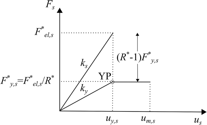

  

  CYD SDOF model seismic response parameters

where F ^* _{el, s} is the elastic strength of the CYD SDOF model and F ^* _{y, s} is the yield strength of the SDOF model, shown in Fig. 3.

The yield displacement u_y,s of the CYD SDOF model is not influenced by the change of its strength F ^* _{y, s} , as presented in Fig. 3. The elastic strength demand is expressed as follows:

$$ F_{el,s}^{*} = m_{s} gC_{el,s}^{*} $$

(5)

where C ^* _{el, s} is the elastic base shear coefficient of the CYD SDOF model, obtained from elastic viscously damped seismic design spectra for a given seismic hazard level.

• 3. Yield stiffness k_y of the CYD SDOF model:

  $$ k_{y} = \frac{{k_{s} }}{{R^{*} }} $$

  (6)

• 4. Elastic vibration period and cyclic frequency of the CYD SDOF model:

  $$ T_{n} = 2\pi \sqrt {\frac{{m_{s} }}{{k_{s} }}} = 2\pi \sqrt {\frac{{m_{s} }}{{F_{el,s}^{*} /u_{y,s} }}} , { }\quad \omega_{n} = \sqrt {\frac{{k_{s} }}{{m_{s} }}} = \sqrt {\frac{{F_{el,s}^{*} /u_{y,s} }}{{m_{s} }}} $$

  (7)

• 5. Yield vibration period and cyclic frequency of the CYD SDOF model:

  $$ T_{y} = 2\pi \sqrt {\frac{{m_{s} }}{{k_{y} }}} = 2\pi \sqrt {\frac{{m_{s} }}{{F_{el,s}^{*} /(R^{*} u_{y,s} )}}} ,\quad \omega_{y} = \sqrt {\frac{{k_{y} }}{{m_{s} }}} = \sqrt {\frac{{F_{el,s}^{*} /(R^{*} u_{y,s} )}}{{m_{s} }}} $$

  (8)

Note that the relation between T_y and T_n is:

$$ T_{y} = T_{n} \sqrt {R^{*} } $$

(9)

• 6. Viscous damping ratio of the CYD SDOF model:

  $$ \xi_{s} = \frac{{c_{s} }}{{2m_{s} \omega_{s} }} $$

  (10)

The inelastic seismic response of the CYD SDOF model is simulated using a bilinear elastic–plastic force–displacement relation, as shown by Tsiavos (2017) and Vassiliou et al. (2013). The yield strength of the CYD SDOF model is (Fig. 3):

$$ F_{y,s}^{*} = k_{y} u_{y,s} $$

(11)

Dynamic equation of motion for the CYD SDOF model with stiffness k_y and strength F ^* _{y, s} (Fig. 3) gives:

$$ \alpha_{s} k_{y} u_{s} + (1 - \alpha_{s} )k_{y} u_{y,s} z_{s} + c_{s} \dot{u}_{s} = - \,m_{s} (\ddot{u}_{g} + \ddot{u}_{s} ) $$

(12)

Using Eq. 6 in Eq. 12 gives:

$$ \alpha_{s} k_{s} u_{s} /R^{*} + (1 - \alpha_{s} )k_{s} u_{y,s} z_{s} /R^{*} + c_{s} \dot{u}_{s} = - \,m_{s} (\ddot{u}_{g} + \ddot{u}_{s} ) $$

(13)

Further, dividing Eq. 13 by m_s gives:

$$ \ddot{u}_{s} = - \,\alpha_{s} \omega_{{_{n} }}^{2} u_{s} /R^{*} - (1 - \alpha_{s} )\omega_{{_{n} }}^{2} u_{y,s} z_{s} /R^{*} - 2\xi_{s} \omega_{n} \dot{u}_{s} - \ddot{u}_{g} $$

(14)

The state space solution of the dynamic equation of motion (Eq. 14) with the modified Bouc–Wen force–displacement relation presented by Tsiavos (2017) and Vassiliou et al. (2013) was performed in Matlab (2012). The dimensionless coefficients controlling the hysteretic behavior of the Bouc–Wen model are β = 0.5, γ = 0.5 and n = 50 to facilitate a sharp transition from the elastic to the inelastic behavior range of the force–displacement response envelope of the CYD SDOF model.

2.1 Dimensional analysis of the CYD SDOF model pulse response

The CYD SDOF structure shown in Fig. 2 is excited by a symmetric Ricker (1943) pulse, defined by Eq. 15 and shown in Fig. 4 as the ground motion acceleration ü_g(t) with a period T_p = 0.5 s and peak acceleration a_p = 0.25 g. The well-defined ground motion characteristics of the Ricker pulse ground motion excitation facilitate its use for dimensional analysis.

Fig. 4

Ricker pulse ground motion excitation with T_p = 0.5 s and a_p = 0.25 g

$$ \ddot{u}_{g} (t) = a_{p} \left( {1 - \frac{{2\pi^{2} (t - 2)^{2} }}{{T_{p}^{2} }}} \right)e^{{ - \frac{1}{2}\frac{{2\pi^{2} (t - 2)^{2} }}{{T_{p}^{2} }}}} $$

(15)

Equation 16 shows that the maximum deformation u_m,s of the CYD SDOF model excited by a Ricker pulse is a function of 7 arguments:

$$ u_{m,s} = f_{1} \left( {T_{n} ,\alpha_{s} ,u_{y,s} ,\xi_{s} ,R^{*} ,a_{p} ,T_{p} } \right) $$

(16)

The yield displacement u_y,s of the CYD SDOF model (Eq. 3) depends on the geometrical characteristics of the model and the mechanical properties of the model yielding material:

$$ u_{y,s} = f_{2} \left( {\varepsilon_{y,s} ,H,\frac{H}{B}} \right) $$

(17)

Following Priestley et al. (2000, 2007), the elastic vibration period T_n of the CYD SDOF model is the shortest vibration period that produces the computed CYD SDOF model yield displacement u_y,s from the symmetric Ricker pulse viscously damped elastic response spectrum, (Fig. 5; Eq. 18). Thus, T_n is a dependent variable.

Fig. 5

Identification of the vibration period T_n of the CYD SDOF model that leads to the chosen value of its yield displacement for a 5% viscously damped elastic displacement response spectrum of a Ricker pulse ground motion excitation with T_p = 0.5 s and a_p = 0.25 g

$$ T_{n} = f_{3} \left( {u_{y,s} ,a_{p} ,T_{p} ,\xi_{s} } \right) $$

(18)

The strength of the CYD SDOF model required for it to remain elastic is obtained using the relation between elastic spectral displacement and pseudo-acceleration is:

$$ F_{el,s}^{*} = m_{s} \left( {\frac{2\pi }{{T_{n} }}} \right)^{2} u_{y,s} $$

(19)

The CYD strength reduction factor R^* is then determined by the yield strength of the CYD SDOF model F ^* _{y, s} using Eq. 4. Finally, displacement ductility demand for the CYD SDOF model subjected to the presented Ricker pulse excitation is a function of 8 variables:

$$ \mu = \frac{{u_{m,s} }}{{u_{y,s} }} = f_{4} (H,{\raise0.7ex\hbox{$H$} \!\mathord{\left/ {\vphantom {H B}}\right.\kern-0pt} \!\lower0.7ex\hbox{$B$}},\varepsilon_{y,s} ,R^{*} ,\alpha_{s} ,\xi_{s} ,a_{p} ,T_{p} ) $$

(20)

Therefore, the principal CYD SDOF model variables that affect its displacement ductility demand are the yield strain of its yielding material, its geometry (height and aspect ratio), the hardening coefficient that defines the post-yielding branch of its force–displacement response envelope, its non-hysteretic (viscous) damping ratio, and the CYD strength reduction factor used to determine its yield strength.

2.2 Comparison of CP and CYD approaches

A steel structure is modeled using the presented CYD SDOF model with H/B = 2, height H = 2 m, mass m_s = 1000t, and an elastic-perfectly-plastic force–deformation response (hardening coefficient α_s = 0). Both models are subjected to a Ricker pulse ground motion excitation with T_p = 0.5 s and a_p = 0.25 g (Eq. 15).

The yield displacement of the CYD SDOF model is u_y,s = 4.8 mm (Eq. 3). Its elastic vibration period is T_n = 0.22 s (Fig. 5) and its elastic strength is F ^* _{el, s}  = 3915.2 kN (Eq. 19). The CP SDOF model of the same structure is assumed to have the same elastic vibration period and elastic strength. The yield strength of both models is set to be the same (F ^* _{y, s}  = F_y,s = 978.8 kN), defined using the CP strength reduction factor R_y = 4 and the CYD strength reduction factor R^* = 4. Note: this yield strength results in the yield displacement of the CP SDOF model u_y,s = F_y,s/k_s = 1.2 mm (Fig. 3).

First, the response of the CYD SDOF model to the symmetric Ricker pulse ground motion excitation is computed by solving its equation of motion (Eq. 14) and plotted in Fig. 6 for a damping ratio value ξ_s = 0. The maximum inelastic displacement of the CYD SDOF model u_m,s = 45.9 mm and the displacement ductility demand µ = 9.56. Then, the response of the constant-period SDOF model to the same excitation is computed by solving its equation motion (Eq. 14) and plotted in Fig. 6. The maximum inelastic displacement of the constant-period SDOF model is u_m,s = 37.9 mm, resulting in a displacement ductility demand µ = 31.6. Even though the displacement response time histories of the two models are similar (Fig. 6), the displacement ductility demand computed using the constant-period approach is significantly higher than that calculated using the CYD approach. This is attributed to the difference between the yield displacements of the two SDOF models.

Fig. 6

Displacement time-history response of the CP and CYD SDOF models for a damping ratio value ξ_s = 0

Force–deformation response of the SDOF models to the Ricker Pulse ground motion are compared in Fig. 7 to show the difference between the constant-period and constant-yield-displacement approaches and to illustrate the role of viscous damping ratio on the inelastic response. The response of the CP SDOF model and the CYD SDOF model differ substantially in their initial stiffness. The effect of non-hysteretic damping ratio ξ_s, 0.001% (for numerical reasons, labeled as 0% in subsequent plots) and 5%, on the inelastic displacement time history response of the SDOF structure with yield strength, subjected to Ricker pulse excitation with T_p = 0.5 s and same yield strength a_p =  0.25 g (Eq. 15) is presented in Fig. 7. The maximum inelastic displacement of the structure with a larger damping value is 18% smaller. This reduction of the inelastic displacement of the structure with increasing non-hysteretic damping values shown in this example is consistent with the observations in Chapter 7 of Chopra (2017). Therefore, the use of very low non-hysteretic damping value to determine the µ–R^*–H/B relation is conservative and the determination of this relation for the displacement-based CYD methodology presented later in this study is based on the use of this low damping value (ξ_s =  0).

Fig. 7

Force-displacement response of the two CP and CYD SDOF models. The response of the CYD SDOF model is computed using two different viscous damping ratios ξ_s = 0.001% (approximately 0%) and ξ_s = 5%

2.3 Comparison of the CP and CYD strength reduction factors

The CYD strength reduction factor R^* defined in this seismic evaluation procedure (Eq. 4; Fig. 3) differs from the CP strength reduction factor R_y (Eq. 1) that is commonly used in seismic design today. The relation between the two strength reduction factors is determined by comparing a CP and a CYD SDOF model with the same yield strength F ^* _{y, s} = F_y,s.

The fundamental difference between the two strength reduction factors is attributed to the different forces required for the two structures to remain elastic (F_el,s and F ^* _{el, s} ), as they are calculated using different vibration periods (namely, T_n and T_y), as presented in Fig. 8. The relation between R^* and R_y can be derived from a pseudo-acceleration design spectrum shown in Fig. 9.

Fig. 8

Comparison of strength reduction factors R^* with R_y

Fig. 9

T_n–T_y period shift shown in a generic pseudo-acceleration design spectrum

Under the assumption that the strengths defined in the two methodologies are the same (F ^* _{y, s} =  F_y,s), and that the periods T_n and T_y are both larger than the corner period T_c of the design spectrum, the strength reduction factor ratio R^*, as presented by Tsiavos (2017) is:

$$ \frac{{R^{*} }}{{R_{y} }} = \frac{{\frac{{F_{el,s}^{*} }}{{F_{y,s}^{*} }}}}{{\frac{{F_{el,s} }}{{F_{y,s} }}}} = \frac{{F_{el,s}^{*} }}{{F_{el,s} }} = \frac{{m_{s} \frac{C}{{T_{n} }}}}{{m_{s} \frac{C}{{T_{y} }}}} = \frac{{T_{y} }}{{T_{n} }} $$

(21)

where C = S_a,maxT_c and S_a,max is the maximum acceleration in the design spectrum (Fig. 9).

Using Eq. 9, Eq. 21 becomes:

$$ \frac{{R^{*} }}{{R_{y} }} = \sqrt {R^{*} } $$

(22)

leading to:

$$ R_{y} = \sqrt {R^{*} } $$

(23)

Similarly, assuming that T_n and T_y are both smaller than the corner period T_c of the design spectrum, the following holds:

$$ R_{y} = R^{*} $$

(24)

3 Constant-R ^* maximum inelastic displacement response spectra

Maximum inelastic displacement spectra for a CYD SDOF model shown in Fig. 2 were determined based on the time history response data obtained by subjecting this CYD SDOF model to a suite of 80 recorded ground motions listed in the “Appendix” (Mackie and Stojadinovic 2005). The ground motion records were obtained from the Pacific Earthquake Engineering Research (PEER) Center next generation attenuation (NGA) strong motion database (PEER 2014). These 80 ground motion records were not scaled, instead they are chosen to represent an ensemble of earthquake ground motion types (near- and far-field), magnitudes (5.5–7.7), and distances (10–60 km). The ground motions were grouped into four bins: a bin with ground motions recorded at small epicentral distance R ranging between 15 and 30 km due to earthquake events with magnitude M_w smaller than 6.5; a bin with ground motions recorded at small epicentral distance (15 km <R < 30 km) due to earthquake events with large magnitude (M_w >  6.5); a bin with ground motions recorded at large epicentral distance (R > 30 km) due to earthquake events with magnitude M_w smaller than 6.5; and a bin with ground motions recorded at large epicentral distance (R > 30 km) due to earthquake events with large magnitude (M_w > 6.5).

Elastic displacement response spectra were computed for each ground motion using a very low value of viscous damping ratio ξ_s = 0.001% (for numerical reasons). Inelastic displacement response spectra were computed using the modified Bouc–Wen force–deformation response model with a bilinear response envelope. As shown in Sect. 2.2, the use of 0% viscous damping for the determination of constant-R^* displacement ductility spectra is conservative, because it leads to the largest displacement ductility demand for the selected force–deformation behavior and the given strength reduction factor R^*.

Then, the average elastic displacement response spectrum for these motions was computed. This spectrum is compared to an Eurocode 8 (CEN, Eurocode 8 Part 1 2004) elastic displacement design spectrum to determine the corner periods T_c and T_d, as shown in Fig. 10.

Fig. 10

Average elastic displacement response spectrum for the 80 ground motions (viscous damping ratio ξ_s = 0.001%) and the fitted EC8 elastic displacement design spectrum

The geometry of the CYD SDOF model, its aspect ratio H/B and height H, and the yield strain of the material ε_y,s are the fundamental design parameters of the CYD SDOF model because they determine the displacement u_y,s of the model (Eqs. 3, 17). Thus, an ensemble of CYD SDOF models was generated by setting the height H, the yield strain of the yielding material ε_y,s (thereby setting the yield displacement), the hardening coefficient α_s and the strength reduction factor R^* and by choosing the values of the aspect ratio H/B from the set{1, 2, …, 10}. Each CYD SDOF model in the ensemble, therefore, had its specific yield displacement, and was examined using the CYD approach (Sect. 2.1) for each one of the 80 ground motions. First, the undamped elastic displacement design spectrum for each ground motion was used to determine the corresponding elastic vibration period T_n of the CYD SDOF model, followed by the calculation of the CYD SDOF elastic strength F ^* _{el, s} . Second, the yield strength F ^* _{y, s} of each of the 10 CYD SDOF models with different aspect ratio H/B values for one ground motion was determined using the selected CYD strength reduction factor R^* to create spectra for a predetermined R^* value (constant-R^* seismic response spectra). Note that the yield strength F ^* _{y, s} is constant for an existing structure, but in order to generate constant-R^* seismic response spectra, the value of yield strength varies in iterations, representing CYD SDOF models with the same geometry, but different strengths. Third, the maximum inelastic displacement of the CYD SDOF models and the corresponding displacement ductility were determined for each of the 80 ground motion records used in this study by solving the equation of motion (Eq. 14) of the CYD SDOF model.

Finally, constant-R^* displacement ductility spectra (the µ–R^*–H/B spectra) for the generated ensemble of CYD SDOF models were constructed by finding the median displacement ductility demand for the 80 ground motions at each considered value of the aspect ratio H/B. An example median R^* = 3 displacement ductility demand spectrum for an ensemble of CYD SDOF models with H = 2 m, ε_y,s = 0.2% and α_s = 0 is shown in Fig. 11a. The yielding material was a structural steel with a nominal yield strength f_y,s = 420 MPa and an elasticity modulus E = 210 GPa. The horizontal line in Fig. 11a indicates the value of the ductility demand derived using the so-called equal displacement rule ($R_{y} = \mu = \sqrt {R^{*} }$) assuming the yield vibration periods of the CYD SDOF models in the ensemble are longer than the elastic response spectrum corner period T_c (Fig. 10).

Fig. 11

a Displacement ductility demand spectra for H = 2 m, f_y,s = 420 MPa and α_s = 0 and R^* = 3; b Displacement ductility spectra for R^* = 2, 3, 4, H = 2 m, f_y,s = 420 MPa and α_s = 0; c Displacement ductility spectra for varying nominal steel yield strength f_y,s values of the yielding material, computed using H = 2 m and α_s = 0 and R^* = 3; d Displacement ductility spectra for varying hardening ratio α_s values computed using H = 2 m and f_y,s = 420 MPa and R^* = 3

The generated CYD SDOF models did not yield (i.e. µ < 1) for a number of combinations of values of its parameters and several records used in this study. Therefore, two median displacement ductility R^* = 3 spectra are plotted in Fig. 11a: one includes only the analyses where yielding occurred, while the other considers all conducted analyses. The percentage of structures that did not experience yielding grows above 10% when the aspect ratio is larger than 5, and exceeds 40% when the aspect ratio is 10. Such slender, deformable structures have a relatively large yield displacement compared to the elastic displacement response spectrum of the selected ground motions (Fig. 10) and do not yield. Henceforth, the data presented in this study pertains only to the events in which the analyzed structure yielded.

The median constant-R^* displacement ductility µ–R^*–H/B spectra for R^* = {2, 3, 4} are shown in Fig. 11b for the CYD SDOF model ensemble with H = 2 m, ε_y,s = 0.2% and α_s = 0. Only the CYD SDOF models that yielded when excited by the ground motions of the 80-motion ensemble were included in the statistical analysis of their maximum response. These values of R^* were selected because they correspond to reasonable values of the conventional strength reduction factor R_y (Eqs. 23 and 24).

Clearly, the ductility demand grows for larger CYD strength reduction factor R^* values. This is expected: in a Yield Point Spectrum approach (Aschheim and Black 2000) the Yield Points of weaker structures are on constant ductility demand capacity spectra with higher displacement ductility. Furthermore, the rate of ductility demand increase becomes larger for structures with smaller aspect ratios. This behavior is a consequence of the shape of a typical pseudo-acceleration design spectrum (Fig. 9). Namely, as the aspect ratio decreases, all other parameters being equal, the yield displacement of the structure is smaller, resulting in shorter elastic and yielding vibration periods T_n and T_y of the CYD SDOF model. Once these periods become smaller than the elastic spectral corner period T_c, where the transition between Eqs. 23 and 24 occurs, the rate of ductility demand change increases.

The median constant R^* = 3 displacement ductility µ–R^*–H/B spectra for two different yield strain values (i.e. ε_y,s = 0.11% and ε_y,s = 0.2% for two different nominal yield strengths of structural steel) are shown in Fig. 11c for the H = 2 m and α_s = 0 ensemble of CYD SDOF models. The µ–R^*–H/B relation is somewhat sensitive to the yield strain value (Eq. 20): smaller yield strains result in smaller yield displacements and shorter vibration periods of the SDOF structures. Therefore, the displacement ductility demand is somewhat larger for structures with smaller yield strains (weaker structural steels). Fortunately, weaker steels are often more ductile than stronger ones. Figure 11d shows the influence of the hardening ratio α_s on the ductility spectra for the H = 2 m ensemble of SDOF structures: this influence is small, indicating that the hardening ratio is not an influential parameter in Eq. 20.

The distributions of the ductility demand values at aspect ratios H/B equal to 1, 5 and 10 for the R^* = 3, H = 2 m, ε_y,s = 0.2% and α_s = 0 ensemble of CYD SDOF models are shown in Fig. 12. The mean and median values of these distributions are listed in Table 1. Lognormal distributions were fit to the response analysis results. The distributions of the ductility demand values (larger than 1) for the investigated aspect ratios are skewed, more so for smaller aspect ratios.

Fig. 12

Displacement ductility spectrum for the CYD SDOF models that yielded (Fig. 11a) and the fitted lognormal distributions for CYD SDOF models with H = 2 m, f_y,s = 420 MPa, α_s = 0 and H/B values of 1, 5 and 10 and R^* = 3

Table 1 Statistical values of displacement ductility demand µ for H/B values of 1, 5 and 10, computed for R^* = 3, H = 2 m, f_y,s = 420 MPa and α_s = 0 CYD SDOF model

Furthermore, a comparison of the medians of the displacement ductility demand values to the so-called equal displacement rule (Table 1) indicates that the inelastic CYD SDOF models displace, on average, less than their equivalent elastic counterparts, and that this difference is growing as the aspect ratio of the CYD SDOF models increases. A similar trend can also be observed in the data presented by Chopra and Chintanapakdee (2001a, b). Therefore, the so-called equal displacement rule is only a conservative approximation of the actual maximum inelastic displacements of a SDOF model.

A strength–ductility–geometry relation that approximates the computed constant-R^* displacement ductility demand µ–R^*–H/B spectra is shown in Fig. 13 and formalized in Eq. 25.

Fig. 13

Displacement ductility spectra for H = 2 m, f_y,s = 420 MPa and α_s = 0 CYD SDOF models (Fig. 11a) and the proposed approximate µ–R^*–H/B relation for R^* = 3

This approximate µ–R^*–H/B relation gives the ductility demand µ related to a CYD strength reduction factor value R^* for an inelastic CYD SDOF model that responds in flexure to earthquake ground motion excitation. The fundamental response behavior of the CYD SDOF investigated in this study is bending. Thus, the proposed approximate µ–R^*–H/B relation does not account for structures with aspect ratios smaller than 1, which are shear dominated.

$$ \mu = \left\{ {\begin{array}{*{20}l} {{\text{not}}\,{\text{applicable}}} \hfill & \quad {H /B \le 1} \hfill \\ {\sqrt {1 + \left( {R^{*} - 1} \right)\frac{{\left( {H /B} \right)_{c} }}{{\left( {H /B} \right)}}} } \hfill & \quad { 1 < H /B \le \left( {H /B} \right)_{c} } \hfill \\ {\sqrt {R^{*} } } \hfill & \quad {H /B\, >\, \left( {H /B} \right)_{c} } \hfill \\ \end{array} } \right. $$

(25)

The critical aspect ratio value (H/B)_c is determined as the aspect ratio value after which the equal displacement rule (µ = $\sqrt {R}$^*) holds. The values of (H/B)_c computed for five different types of construction steel (i.e. five different yield strain ε_y,s values) and three values of the structure force–displacement response hardening coefficient α_s = {0, 5%, 10%} are shown in Table 2. The critical aspect ratio values are presented as dimensionless ratios of predetermined values given in meters (either 4 m or 5 m) to the height of the CYD SDOF model H, also expressed in meters. For example, the critical aspect ratio of a CYD SDOF model with H = 3 m, α_s = 0, f_y,s = 235 MPa and R* = 2 is 5 m/3 m = 1.67. The values of (H/B)_c in Eq. 25 for the intermediate values of the CYD SDOF model response parameters can be linearly interpolated using the values in Table 2.

Table 2 Non-dimensional (H/B)_c values for varying values of CYD SDOF model strength reduction factor R^*, force–deformation response hardening ratio α_s and nominal steel yield strengths f_y,s with H also expressed in meters

The critical aspect ratio (H/B)_c is inversely proportional to the height of the CYD SDOF model. Taller models are more deformable and have larger yield displacements for the same aspect ratio H/B value (Eq. 3). Similarly, CYD SDOF models with stronger steel yielding materials have larger yield strains, resulting in larger yield displacements for the same aspect ratio H/B value. Thus, the displacement ductility demand μ developed by these models is smaller (for the same aspect ratio H/B value). Consequently, the value of the critical aspect ratio (H/B)_c, after which the equal displacement rule ($\mu = \sqrt {R^{*} }$) holds, is smaller. Higher values of hardening α_s lead to a less significant reduction of the displacement ductility demand μ (for the same aspect ratio value H/B), thus decreasing the value of the critical aspect ratio (H/B)_c in a similar way. The value of this critical aspect ratio (H/B)_c is independent from the value of the CYD strength reduction factor R^* (Fig. 11b): this was similarly shown by Chopra and Chintanapakdee (2001b) for various values of the strength reduction factor R_y.

Based on the data in Table 2, the hyperbolic portion of the µ–R^*–H/B relations vanishes for practically all SDOF structures with heights H >  4 m. Only for structures with relatively weak steels (small yield strains) the hyperbolic portion of the proposed µ–R^*–H/B relation remains. In such cases, it becomes shorter when the hardening coefficient α_s increases. To show this, the proposed µ–R^*–H/B relations (Eq. 25) for R^* = 4, nominal steel yield strength f_y,s = 235 MPa (yield strain ε_y,s =  0.11%), and hardening ratio α_s = 0 are plotted in Fig. 14 for three different values of the CYD SDOF model height H = {1, 2, 4} m.

Fig. 14

Proposed approximate µ–R^*–H/B relations for varying heights H (m), with the strength reduction factor R^* = 4, f_y,s = 235 MPa and α_s = 0, i.e. (H/B)_c = 5 m/H

4 Constant yield displacement seismic evaluation procedure

The approximate µ–R^*–H/B relations for CYD SDOF models make it possible to develop a displacement-based seismic performance evaluation procedure for existing structures that respond to ground motion excitation predominantly in flexure, the Constant Yield Displacement Evaluation (CYDE) procedure. The intent is to parallel the conventional non-linear static seismic evaluation procedures based on maximum inelastic displacement estimates, such as those developed by Ruiz-García and Miranda (2003) and implemented in ASCE 41-13 (2013), or yield strength estimates obtained using conventional R_y–µ–T_n relations and implemented in numerous evaluation and design procedures as discussed in Chopra (2017).

Starting from the basic parameters of an existing structure, namely its geometry (height, aspect ratios, areas), the mechanical characteristics of its yielding material, and its mass and mass distribution, the goal of the CYDE procedure is to determine the displacement ductility demand µ for the existing structure subjected to earthquake ground motion excitations expected for the seismic hazard level the structure is evaluated at, and compare it to the displacement ductility capacity of the existing structure to determine if this structure is satisfactory.

The CYDE procedure to determine the displacement ductility demand for a given seismic hazard level comprises the following steps (Fig. 15):

Fig. 15

Steps of the CYDE procedure

• 1. Determine the properties of the CYD SDOF model of the existing structure: Following the procedure developed by Tjhin et al. (2007), based on a fundamental vibration mode equivalent SDOF system, determine the effective height H, the yield displacement u_y,s, the participating seismic mass m_s and the yield strength F ^* _{y, s} of the CYD SDOF model.

• 2. CalculateF ^* _{el, s} , the strength required for this CYD SDOF model to remain elastic for the given design seismic hazard. This can be done in two ways. First, using the viscously undamped elastic displacement seismic response spectrum for the evaluated seismic hazard level, find the shortest elastic vibration period T_n corresponding to the calculated yield displacement u_y,s as shown in Fig. 5, and then use Eq. 19. Alternatively, construct the viscously undamped elastic capacity response spectrum for the considered seismic hazard level and, starting with the CYD SDOF yield displacement, read the desired elastic base shear coefficient C ^* _{el, s} directly, then multiply by the seismic weight as in Eq. 5.

• 3. DetermineR^*, the strength reduction factor of the CYD SDOF model using the yield strength F ^* _{y, s} using Eq. 4.

• 4. Calculate the displacement ductility demandµ of the structure from the µ–R^*–H/B relations (Eq. 25) and the maximum inelastic displacement u_m,s from Eq. 2. Obtain an elastic-perfectly-plastic force–displacement response of the CYD SDOF system and convert it back to the model of the existing structure using the Tjhin et al. (2007) procedure. Compare the obtained displacement ductility demand (or maximum inelastic displacement) to the expected displacement ductility capacity of the existing structure and determine if it satisfies the performance objective(s) for the selected seismic hazard level.

4.1 Comparison of the CYD µ–R ^*–H/B relations and test data

The CYD µ–R^*–H/B approximate relations represent the constant-R* seismic response spectra for a CYD SDOF derived using a statistical rendering of the time history response data obtained using an ensemble of 80 recorded ground motions (“Appendix”). Here the displacement ductility demand estimated using the proposed µ–R^*–H/B relation (Eq. 25) is compared to the results obtained from a large-scale shake table test of a 3-storey reinforced concrete shear wall completed by Lestuzzi and Bachmann (2007). The 3-story structure WDH1 shown in Fig. 16 has a height of 4.3 m, an effective height of the first-mode equivalent CYD SDOF model (Tjhin et al. 2007) H = (0.833)·4.3 m = 3.58 m and a width of 1.00 m, making the aspect ratio H/B = 3.58. The participating mass of the CYD SDOF model is m_s = 35.87t. The strength of the steel reinforcement is f_y,s = 500 MPa. The yield displacement of the structure determined using Eq. 3 is u_y,s = 20.34 mm.

In the test, the structure was subjected to a synthetic ground motion simulating a design earthquake valid for the most severe seismic zone (Zone 3b) of the Swiss Earthquake Code SIA 160 (1989) for a peak ground acceleration of 1.6 m/s². The elastic spectral acceleration for this structure is S_a(u_y,s = 23.7 mm) = 0.34 g, based on a SIA 160 elastic design spectrum with 10% probability of exceedance in 50 years. Then, the elastic strength is F ^* _{el, s}  = 358.7 kN·0.34 = 122 kN. The base shear yield strength of the tested wall was not measured directly, so it is estimated in two ways. First, the experimentally derived yield vibration period of the structure T_y = 0.8 s, resulting in the yield strength of the structure being F ^* _{y, s}  = k_y·u_y,s = m_s·(2π/T_y)²·u_y,s = 45 kN, and the strength reduction factor R^* = 2.71 (Eq. 4). Second, using the nominal bending strength of the structure M_y = 157.5 kNm (Lestuzzi and Bachmann 2007) and a linear first-mode lateral force distribution, the yield strength of the structure F ^* _{y, s}  = 43.4 kN, resulting in a strength reduction factor R^* = 2.81. The critical aspect ratio is (H/B)_c = 1.12 (Table 2). Using the proposed µ–R^*–H/B relations (Eq. 25), the displacement ductility demand estimates for the presented structure are µ = $\sqrt {R}$^* = 1.65 and 1.68, respectively. The ductility demand µ observed during the test was 1.5 (Lestuzzi and Bachmann 2007). Thus, the estimates of the specimen displacement ductility demand computed using the µ–R^*–H/B relations are in good agreement with the experimental results. They are slightly larger, thus on the conservative side, as intended by the derivation of the µ–R^*–H/B relations.

Fig. 16

A 3-storey reinforced concrete shear wall tested by Lestuzzi and Bachmann (2007)

4.2 Application of the CYDE procedure

A symmetric four-story reinforced concrete building with a total height H_w = 11.2 m (floor height is 2.8 m) and seismic mass m_s,total = 4·335t = 1340t is seismically designed using four reinforced concrete shear walls of the same cross-section (Fig. 17). For this existing building a life-safety limit state, the roof-level displacement ductility capacity of the walls is estimated at 2.0. The steel reinforcement yield strength is f_y,s = 420 MPa. The vertical reinforcement, relevant for flexural resistance of the shear walls, is assumed to be concentrated in the boundary elements. The total reinforcement area in one boundary element A = 0.00723 m², and the distance between the centroids of these areas is B = 1.4 m (Fig. 17). Following the CYDE procedure in Fig. 15, the effective height of this CYD SDOF model H = 0.816 H_w = 9.14 m (Tjhin et al. 2007), the aspect ratio is H/B = 6.53 and the yield displacement of the CYD SDOF model is u_y,s = 0.08 m (Eq. 3).

Fig. 17

Transformation of a MDOF model of a structure to a CYD SDOF model

The participating mass of the CYD SDOF model is m_s = $\sum\nolimits_{i = 1}^{4} {m_{i} \phi_{i1} }$ = 837.5t, where m_i = 335t is the mass of the ith floor and φ_i1 is the first mode shape (assumed as linear for this example) amplitude at the ith floor. The yield strength of the building is V_y,s = 2V_y,wall in each of the horizontal directions (V_y,wall = f_y,sAB/H = 465.65 kN is the flexural strength of each wall). The yield strength of the CYD SDOF model is F ^* _{y, s}  = (m_s/m_s,total)V_y,s/α₁ = 0.88V_y,s = 819.55 kN, where α₁ = 0.707 is the effective modal mass coefficient for the first mode (Tjhin et al. 2007). The elastic base shear coefficient corresponding to the CYD SDOF yield displacement of 0.08 m is C ^* _{el, s}  = 0.4, as shown in the design capacity spectrum shown in Fig. 17. Consequently, the base shear strength of the CYD SDOF model such that remains elastic for the considered seismic hazard level is F ^* _{el, s}  = 837.5t·9.81 m/s²·0.4 = 3286.35 kN, resulting in a CYD strength reduction factor R^* = 4. The critical aspect ratio is (H/B)_c = 0.44 (Table 2). Using the µ–R^*–H/B relation (Eq. 25), the estimate of the CYD SDOF ductility demand µ = $\sqrt {R}$^* = 2. The CYD SDOF estimate of the displacement ductility demand remains unchanged through the transformation to the building MDOF model. Evidently, the existing building meets the life safety performance objective (displacement ductility demand = displacement ductility capacity).

5 Conclusions

Seismic performance evaluation is an important task conducted often in design offices simply because a large majority of the built inventory of a typical established community is already there and exposed to seismic hazard. The non-linear static seismic evaluation procedure is the method of choice for many engineers because of a favorable balance between the quality of the obtained information about the behavior of an existing structure and the complexity of performing the evaluation. Practically all such procedures represent the seismic response of the existing structure using a corresponding single-degree-of-freedom model. In addition, many non-linear static procedures are based on relations between the strength of the structure, the deformation ductility of the structure and the fundamental vibration period of the structure (R_y–μ–T_n relations) derived using an assumption that the period of the structure remains constant as its strength is varied.

A different approach was taken in this paper. It is based on the fact that the yield displacement of a structure depends on its geometry and mechanical properties of its yield material, and is also constant for an existing structure. The so-called constant-yield-displacement approach was developed first, and used to compute the inelastic earthquake response spectra of the CYD SDOF model of an existing structure. In the process, a new strength reduction factor R^* was defined in accordance with the constant yield displacement assumption. Then, constant-R^* inelastic displacement ductility seismic response spectra, parametrized by the geometry and the yield strain of the CYD SDOF model, were developed by statistical rendering of the results of non-linear time history analyses of CYD SDOF model seismic responses to an ensemble of 80 recorded ground motions. These µ–R^*–H/B seismic response spectra make it possible to determine the displacement ductility demand, and thus the maximum inelastic displacement, of the CYD SDOF model of an existing structure.

A novel Constant Yield Displacement Evaluation (CYDE) procedure for seismic evaluation of existing structures was proposed. Based on the values of the yield displacement and the yield strength of the CYD SDOF model of an existing structure, which can be determined with confidence for many existing structures, and the seismic hazard the structure is evaluated for, the CYDE procedure provides an estimate of the displacement ductility demand the structure is likely to experience. This ductility demand can be compared to the ductility capacity of an existing structure to determine if it meets the required performance objective or not. The four-step CYDE procedure was demonstrated in a simple example, showing that it is similar to the existing constant-period-based seismic evaluation procedures and easy to do.

The principal advantage of the CYDE seismic evaluation procedure is that the fundamental vibration period of the structure is derived from estimates of its yield displacement and yield strength. Thus, estimates of the fundamental vibration period, i.e. the stiffness, of the structure are not needed in the evaluation procedure. Another advantage is that the µ–R^*–H/B response spectra do not vary dramatically across the range of CYD SDOF aspect ratio values and are predictably sensitive to the changes in the yield strength of the structure. This makes the CYDE seismic evaluation procedure fairly stable in the face of possible errors in the estimate of geometric and mechanical properties of the evaluated structure.

The shortcomings of the developed µ–R^*–H/B relations and the CYDE procedure stem from the assumptions made about the behavior of the CYD SDOF model. First, the CYD SDOF model was assumed to respond in flexure. Thus, the µ–R^*–H/B relations should be used with caution for CYD SDOF model aspect ratios H/B < 2 and do not apply for aspect ratios H/B < 1. For CYD SDOF models with H/B < 1, new µ–R^*–H/B relations should be developed to account for the shear or the sliding inelastic response. Second, the proposed µ–R^*–H/B relations were developed using the bilinear elastic–plastic force–displacement response model. This model provides a good balance between the ability to simulate the critical aspects of the dynamics of the evaluated structure and the simplicity needed to automate the analysis of the response of the structure for a wide range of ground motion excitations. However, other force–displacement response models, in particular those with pinched hysteresis loops and degrading response envelopes should be investigated to determine if and how they affect the proposed µ–R^*–H/B relations. Finally, the proposed CYDE procedure needs to be applied to a wider variety of structures with different lateral load resisting systems and materials as well as geometric irregularities in order to demonstrate its robustness. Work to overcome these shortcomings is ongoing.

Appendix

See Table 3.

Table 3 Earthquake ground motions ensemble used to develop the µ–R^*–H/B relations

References

ASCE 31–03 (2003) Seismic evaluation of existing buildings. American Society of Civil Engineers, Reston
ASCE 41-06 (2006) Seismic rehabilitation of existing buildings. American Society of Civil Engineers, Reston
ASCE 41-13 (2013) Seismic evaluation and upgrade of existing buildings. American Society of Civil Engineers, Reston
ASCE 41-17 (2017) Seismic evaluation and upgrade of existing buildings. American Society of Civil Engineers, Reston
Aschheim M (2002) Seismic design based on the yield displacement. Earthq Spectra 18(4):581–600
Aschheim M, Black EF (2000) Yield point spectra for seismic design and rehabilitation. Earthq Spectra 16(2):317–335
Beyer K, Simonini S, Constantin R, Rutenberg A (2014) Seismic shear distribution among interconnected cantilever walls of different lengths. Earthq Eng Struct Dyn 43(10):1423–1441
CEN, Eurocode 8 Part 1 (2004) Design of structures for earthquake resistance part 1: general rules, seismic actions and rules for buildings, EN 1998-1:2004. Comite Europeen de Normalisation, Brussels
CEN, Eurocode 8 Part 3 (2004) Design of structures for earthquake resistance part 1: assessment and retrofitting of buildings, EN 1998-3:2004. Comite Europeen de Normalisation, Brussels
Chopra AK (2017) Dynamics of structures: theory and applications to earthquake engineering, 5th edn. Prentice-Hall, Englewood Cliffs
Chopra AK, Chintanapakdee C (2001a) Comparing response of SDF systems to near-fault and far-fault earthquake motions in the context of spectral regions. Earthq Eng Struct Dyn 30(12):1769–1789
Chopra AK, Chintanapakdee C (2001b) Inelastic deformation ratios for design and evaluation of structures: single-degree-of-freedom bilinear systems. J Struct Eng 130:1309–1319
Elghadamsi FE, Mohraz B (1987) Inelastic earthquake spectra. Earthq Eng Struct Dyn 15:91–104
Lestuzzi P, Bachmann H (2007) Displacement ductility and energy assessment from shaking table tests on RC structural walls. Eng Struct 29(8):1708–1721
Mackie KR, Stojadinovic B (2005) Fragility basis for California highway overpass bridge seismic decision-making. PEER report 2005/02, Pacific Earthquake Engineering Research Center, University of California, Berkeley
Matlab (2012) MATLAB and statistics toolbox release. The Mathworks Inc., Natick
Miranda E (1993) Evaluation of site-dependent inelastic seismic design spectra. J Struct Eng 119(5):1319–1338
Miranda E, Bertero VV (1994) Evaluation of strength reduction factors for earthquake resistant design. Earthq Spectra 10:357–379
Nassar AA, Krawinkler H (1991) Seismic demands for SDOF and MDOF systems. Report 95, The John A. Blume Earthquake Engineering Center, Stanford University, Stanford
Newmark NM, Hall WJ (1973) Seismic design criteria for nuclear reactor facilities. Report 46, Building Practices for Disaster Mitigation, National Bureau of Standards
PEER NGA Strong Motion Database (2014) Pacific earthquake engineering research center, University of California, Berkeley. http://peer.berkeley.edu/nga/. Accessed 08 Sept 2014
Priestley MJN (2000) Performance based seismic design. In: Proceedings of the 12th world conference on earthquake engineering, New Zealand
Priestley MJN, Calvi GM, Kowalsky MJ (2000) Direct displacement-based seismic design of concrete buildings. Bull N Z Soc Earthq Eng 33(4):421–444
Priestley MJN, Calvi GM, Kowalsky MJ (2007) Displacement based seismic design of structures. IUSS, Pavia
Ricker N (1943) Further developments in the wavelet theory of seismogram structure. Bull Seismol Soc Am 33:197–228
Riddell R, Hidalgo PA, Cruz EF (1989) Response modification factors for earthquake resistant design of short period buildings. Earthq Spectra 5(3):571–590
Ruiz-García J, Miranda E (2003) Inelastic displacement ratios for evaluation of existing structures. Earthq Eng Struct Dyn 32:1237–1258. https://doi.org/10.1002/eqe.271
SIA 160 (1989) Einwirkung auf Tragwerke. Schweiz. Ingenieur-und Architekten-Verein, Zurich
Sollogoub P (1994) Inelastic behavior of structures on aseismic isolation pads. In: Tenth European conference on earthquake engineering, Vienna, Austria
Tjhin TN, Aschheim MA, Wallace JW (2007) Yield displacement-based seismic design of RC wall buildings. Eng Struct 29:2946–2959
Tsiavos A (2017) New approaches for the performance-based design of conventional and seismically isolated structures, Ph.D. dissertation, ETH Zurich
Tsiavos A, Vassiliou MF, Mackie KR, Stojadinovic B (2013a) R–μ–T relationships for seismically isolated structures. In: COMPDYN 2013, 4th international conference on computational methods in structural dynamics and earthquake engineering, Kos Island, Greece
Tsiavos A, Vassiliou MF, Mackie KR, Stojadinovic B (2013b) Comparison of the inelastic response of base-isolated structures to near-fault and far-fault ground motions. In: VEESD 2013, Vienna congress on recent advances in earthquake engineering and structural dynamics & D-A-CH Tagung, Vienna, Austria
Tsiavos A, Mackie KR, Vassiliou MF, Stojadinovic B (2017) Dynamics of inelastic base-isolated structures subjected to recorded ground motions. Bull Earthq Eng 15(4):1807–1830
Vassiliou MF, Tsiavos A, Stojadinovic B (2013) Dynamics of inelastic base-isolated structures subjected to analytical pulse ground motions. Earthq Eng Struct Dyn 42(14):2043–2060
Veletsos AS, Newmark NM (1960) Effect of inelastic behavior on the response of simple systems to earthquake motions. In: Proceedings of the 2nd world conference on earthquake engineering, Japan, vol 2, pp 895–912
Veletsos AS, Newmark NM, Chelapati CV (1965) Deformation spectra for elastic and elastoplastic systems subjected to ground shock and earthquake motions. In: Proceedings of the 3rd world conference on earthquake engineering, New Zealand, vol II, pp 663–682
Vidic T, Fajfar P, Fischinger M (1994) Consistent inelastic design spectra: strength and displacement. Earthq Eng Struct Dyn 23:502–521
Funding
Funding was provided by ETH Zurich.
Author information
Authors and Affiliations
Corresponding author
Additional information
Publisher's Note
Springer Nature remains neutral with regard to jurisdictional claims in published maps and institutional affiliations.
Appendix
See Table 3.
Rights and permissions
OpenAccess This article is distributed under the terms of the Creative Commons Attribution 4.0 International License (http://creativecommons.org/licenses/by/4.0/), which permits unrestricted use, distribution, and reproduction in any medium, provided you give appropriate credit to the original author(s) and the source, provide a link to the Creative Commons license, and indicate if changes were made.
About this article
Cite this article
Tsiavos, A., Stojadinović, B. Constant yield displacement procedure for seismic evaluation of existing structures. Bull Earthquake Eng 17, 2137–2164 (2019). https://doi.org/10.1007/s10518-018-00532-w
Received:
Accepted:
Published:
Issue Date:
DOI: https://doi.org/10.1007/s10518-018-00532-w