GoCo: planning expressive commitment protocols

Abstract

This article addresses the challenge of planning coordinated activities for a set of autonomous agents, who coordinate according to social commitments among themselves. We develop a multi-agent plan in the form of a commitment protocol that allows the agents to coordinate in a flexible manner, retaining their autonomy in terms of the goals they adopt so long as their actions adhere to the commitments they have made. We consider an expressive first-order setting with probabilistic uncertainty over action outcomes. We contribute the first practical means to derive protocol enactments which maximise expected utility from the point of view of one agent. Our work makes two main contributions. First, we show how Hierarchical Task Network planning can be used to enact a previous semantics for commitment and goal alignment, and we extend that semantics in order to enact first-order commitment protocols. Second, supposing a cooperative setting, we introduce uncertainty in order to capture the reality that an agent does not know for certain that its partners will successfully act on their part of the commitment protocol. Altogether, we employ hierarchical planning techniques to check whether a commitment protocol can be enacted efficiently, and generate protocol enactments under a variety of conditions. The resulting protocol enactments can be optimised either for the expected reward or the probability of a successful execution of the protocol. We illustrate our approach on a real-world healthcare scenario.

1 Introduction

Modern information technology (IT) applications in a variety of domains involve interactions between autonomous parties such as people and businesses. For example, IT serves a pivotal role for the patients, staff, departments, and stakeholders in a modern healthcare centre [40]. The field of multi-agent systems provides constructs to deal with such settings through the notions of autonomous agents and their protocols of interaction. However, many challenges remain to building a realistic multi-agent society.

In particular, agents in a system, although autonomous, may be interdependent in subtle ways. The physical, social, or organisational environment in which they interact can be complex. We need ways to accommodate the environment while supporting decoupling of the agents’ internals from their interaction, thus facilitating the composition of multi-agent systems. The notion of a socio-technical system (STS) [23, 58] provides a basis for representing such interactions between agents in the context of an organisation, such as a healthcare centre, and respecting technical artefacts required for the effective operation of the organisation. Here, activities in an STS are characterised by a combination of the goals sought by and the specified interactions between the agents.

Along these lines, the notion of (social) commitments [54,55,56] has been adopted to describe interactions among agents in a high-level implementation-independent manner. A particularly important feature of commitments is that they are a public construct in that they define a relationship between the concerned parties. Of course, any party may represent a commitment internally but the meaning and significance of commitments derives from their relational nature. Over the years, there has been progress on structuring interactions in terms of commitment protocols [7, 8, 19, 20, 25, 35, 69]. Commitment protocols offer a noted advantage in that they enable participating agents to coordinate in a flexible manner, retaining their autonomy. An agent would comply with a protocol as long as it does not violate any of its commitments—thus, in general, an agent may act in a variety of compliant ways to satisfy its goals. Once stakeholders design a commitment protocol, it is then up to the individual agents to instantiate commitments operationally in order to achieve their individual goals [23].

Put another way, goals relate to commitments at two levels: at design time, the collaborative design process produces a commitment protocol; and at run time, agents consider the protocol and their respective goals and make their decisions accordingly. This view leads us to two main challenges:

• Where do the protocols come from? Collaborative organisational design and redesign involve stakeholders jointly exploring the specification of a socio-technical system in terms of the goals and commitments of the individual agents participating in the STS. Previous work examined this problem qualitatively, for example, through Protos [18], an abstract design process for capturing requirements of multiple stakeholders through an STS specification constructed in terms of commitments (with its associated formal assumptions).

• How can an agent gain assurance that its goals are indeed achievable when the STS is instantiated? An important challenge is to specify an STS so that autonomous agents with their individual goals would want to participate in it—that is, to provide an assurance to the agents that their participation would lead to their goals being satisfied.

Our contribution is to address the foregoing challenges by moving from a purely qualitative generated specification to one that allows the verification of the properties of actual instantiations of the commitment protocols. While previous approaches have addressed the challenge of whether a protocol can be verified in the sense that participants can enforce it [7] (i.e., observe that agents comply with it), we address a more fundamental question of whether a protocol can be enacted in the environment for which it was designed. Specifically, the problem we address is the design of commitment protocols for agents acting in uncertain environments, and the validation of the feasibility of the commitment protocol from a centralised perspective.

Our planning-based approach provides a computational mechanism to reason about a number of properties of commitment protocols and their enactments. In this article, we consider an enactment to be an instantiation of a protocol defined in terms of goals and commitments that corresponds to the full hierarchical decomposition of an Hierarchical Task Network (HTN) task using a method library [29], simply put, an enactment is a sequence of executable actions that fulfills agent goals and satisfies their commitments. An enactment is optimal if it maximises the expected utility [12] across all alternative enactments. First, we can identify whether or not a commitment protocol is compatible with the agent’s goals, i.e., whether there is at least one enactment of the protocol that achieves one or more individual goals. Second, our approach can quickly generate a suboptimal enactment to prove a protocol is feasible as well as generate all possible enactments, if needed. Third, we can provide a quantitative assessment of the utilities of each possible enactment of the commitment protocol. Fourth, we can use the exhaustive generation of enactments to select among them regarding their utility to one or more of the participating agents.

Our previous work provided the initial steps to automate the verification of the realisability of instances of commitment protocols using planning formalisms [50, 62] as well as quantifying the utility of such instances [51]. This article consolidates these contributions and provides five novel contributions. First, we formalise a typical socio-technical system, namely a real-world healthcare scenario (introduced in Sect. 2 and formalised in Sect. 5), that is used throughout the article to illustrate the approach, and which can be used to test the scalability of approaches such as ours. Second, in Sect. 3 (augmented by Sect. 4.1) we provide a complete account of the planning formalism used to reason about commitment protocols and how they relate to individual agent goals. This formalisation extends our previous work by providing a probabilistic view of the environment and the utilities of states, allowing the algorithms that generate possible enactments to reason about their expected utilities. Third, in Sect. 4 we provide the complete extended formalisation of the commitment dynamics and reasoning patterns [63] underlying our verification system. Fourth, in Sect. 6 we develop a depth-first search algorithm, ND-PyHop, to explore commitment protocols in stochastic environments and generate realisable protocol enactments. We show that using ND-PyHop we can generate protocol enactments that satisfy a minimal expected utility criterion in exponential time and linear memory. Finally, in Sect. 7 we evaluate the efficiency of the resulting approach for increasingly complex instantiations of the healthcare scenario. We conclude the article with a discussion of related research and future directions.

2 Healthcare scenario

Throughout this article, we use the following scenario as an example of the application of our contribtuion. The scenario is illustrative and useful for two reasons. First, it shows a complex network of commitment between a number of parties/agents that would be ill-suited to model as a monolithic system, showcasing the power of modelling systems in terms of multiple interacting agents following commitment protocols. Second, it is amenable to generating arbitrarily large instantiations as the number of instances of agent roles (e.g., physicians, patients, and radiologists), enabling it to be employed in empirical experimentation to measure the scalability of the algorithms we develop.

Fig. 1

A breast cancer diagnosis process [3]

The scenario is drawn from a real-world healthcare application domain. Figure 1 shows a breast cancer diagnosis process adapted from a report produced by a U.S. governmental committee [3]. We omit the tumour board, which serves as an authority to resolve any disagreements among the participants. For readability, we associate feminine pronouns with the patient, radiologist, and registrar, and masculine pronouns with the physician and pathologist.¹

The process begins when the patient (not shown in the figure) visits a primary care physician, who detects a suspicious mass in her breast. He sends the patient over to a radiologist for mammography. If the radiologist notices suspicious calcifications, she sends a report to the physician recommending a biopsy. The physician requests the radiologist to perform a biopsy, who collects a tissue specimen from the patient, and sends it to the pathologist. The pathologist analyses the specimen, and performs ancillary studies. If necessary, the pathologist and radiologist confer to reconcile their findings and produce a consensus report. The physician reviews the integrated report with the patient to create a treatment plan. The pathologist forwards his report to the registrar, who adds the patient to a state-wide cancer registry that she maintains.

We formalise this scenario in the next sections and use it as an example in the rest of the article.

3 Formal background

Here we introduce the fundamental background upon which we build our formalisation of planning for commitment protocols. Section 3.1 defines the first-order logic language we use to formally represent agent goals and commitments, and the planning operators with which the agents reason about the realisation of the commitment protocols. We review the propositional formalisation of commitments from Telang et al. [63] in Sect. 3.2, from which (in Sect. 4) we will build a first-order operationalisation from Meneguzzi et al.  [50] that can handle different instances of the same commitment. Finally, in Sect. 3.3 we introduce the planning formalism we subsequently extend in Sect. 4.1 and employ thereafter.

3.1 Formal language and logic

Our formal language is based on first-order logic and consists of an infinite set of symbols for predicates, constants, functions, and variables. It obeys the usual formation rules of first-order logic and follows its usual semantics when describing planning domains [32].

Definition 1

(Term) A term, denoted generically as $\tau$, is a variable following the prolog convention of an uppercase starting letter $A,B, \dots , Z, \dots$ (with or without subscripts); a constant a, b, c (with or without subscripts); or a function term $f(\tau _0,\ldots ,\tau _n)$, where f is a n-ary function symbol applied to (possibly nested) terms $\tau _0,\ldots ,\tau _n$.

Definition 2

(Atoms and formulas) A first-order atomic formula (or atom), denoted as $\varphi$, is a construct of the form $p(\tau _0,\ldots ,\tau _n)$, where p is an n-ary predicate symbol and $\tau _0,\ldots ,\tau _n$ are terms. A first-order formula $\varPhi$ is recursively defined as $\varPhi ::= \varPhi \wedge \varPhi ' | \lnot \varPhi | \varphi$. A formula is said to be ground, if it contains no variables or if all the variables in it are bound to a constant symbol.

We assume the usual abbreviations: $\varPhi \vee \varPhi '$ stands for $\lnot (\lnot \varPhi \wedge \lnot \varPhi ')$; $\varPhi \rightarrow \varPhi '$ stands for $\lnot \varPhi \vee \varPhi '$ and $\varPhi \leftrightarrow \varPhi '$ stands for $(\varPhi \rightarrow \varPhi ') \wedge (\varPhi '\rightarrow \varPhi )$. Additionally, we also adopt the equivalence $\{\varPhi _1,\ldots ,\varPhi _n\}\equiv (\varPhi _1\wedge \cdots \wedge \varPhi _n)$ and use these interchangeably. Our mechanisms use first-order unification [2], which is based on the concept of substitutions.

Definition 3

(Substitution) A substitution $\sigma$ is a finite and possibly empty set of pairs $\{x_1/\tau _1,\ldots , x_n/\tau _n\}$, where $x_1,\ldots ,x_n$ are distinct variables and each $\tau _i$ is a term such that $\tau _i \ne x_i$.

Given an expression E and a substitution $\sigma = \{x_1/\tau _1, \ldots ,x_n/\tau _n\}$, we use $E\sigma$ to denote the expression obtained from E by simultaneously replacing each occurrence of $x_i$ in E with $\tau _i$, for all $i \in \{1,\ldots ,n\}$.

Substitutions can be composed; that is, for any substitutions $\sigma _1=\{x_1/\tau _1,\ldots ,x_n/\tau _n\}$ and $\sigma _2=\{y_1/\tau '_1,\ldots ,y_k/\tau '_k\}$, their composition, denoted as $\sigma _1 \cdot \sigma _2$, is defined as $\{x_1/(\tau _1\cdot \sigma _2),\ldots ,x_n/(\tau _n\cdot \sigma _2), z_1/ (z_1 \cdot \sigma _2), \ldots , z_m/ (z_m \cdot \sigma _2)\}$, where $\{z_1,\ldots ,z_m\}$ are those variables in $\{y_1,\ldots ,y_k\}$ that are not in $\{x_1,\ldots ,x_n\}$. A substitution $\sigma$ is a unifier of two terms $\tau _1,\tau _2$, if and only if $\tau _1\cdot \sigma = \tau _2\cdot \sigma$.

Definition 4

(Unify Relation) Relation $unify (\tau _1,\tau _2,\sigma )$ holds iff $\tau _1\cdot \sigma = \tau _2\cdot \sigma$. Moreover, $unify (p(\tau _0, \ldots , \tau _n),p(\tau '_0,\ldots ,\tau '_n),\sigma )$ holds iff $unify (\tau _i,\tau '_i,\sigma ),$ for all $0\le i\le n$.

Thus, two terms $\tau _1,\tau _2$ are related through the $unify$ relation if there is a substitution $\sigma$ that makes the terms syntactically equal. The logic language is used to define a state within a planning domain, as follows:

Definition 5

(State) A state is a finite set of ground atoms (facts) that represent logical values according to some interpretation. Facts are divided into two types: positive and negated facts, as well as constants for truth ($\top$) and falsehood ($\bot$).

3.2 Goal and commitment operational semantics

We adopt the notion of a (social) commitment, which describes an element of the social relationships between two agents in high-level terms. A commitment in this article is not to be confused with a ‘psychological’ commitment expressing an agent’s entrenchment with its intentions [16, 54, 57]. Commitments are extensively studied in multi-agent systems [27, 31, 65] and are traditionally defined exclusively in terms of propositional logic constructs. Recent commitment-query languages, e.g., [21, 22], go beyond propositional constructs but do not address the challenges studied in this article.

We make a distinction between commitment templates (which describe commitments in general) and commitment instances, which allow for variable bindings that differentiate commitments adopted by specific parties and referring to specific objects in the domain. Although we elaborate on the formalisation of commitment instances in Sect. 4.2, we represent commitment template tuples exactly as the commitment formalisation of Telang et al. [63] and define commitment instances later in the article. Thus, in this section, we explain the commitment formalism in a simplified manner before extending it to handle multiple commitment instances and the additional formalism required to reason with them.

A commitment $\mathsf {C}$(de, ct, antecedent, consequent) means that the debtor agent de commits to the creditor agent ct to bring about the consequent if the antecedent holds [56]. Figure 2 summarises a commitment lifecycle [63]. Upon creation, a commitment transitions from state null to active, which consists of two substates: conditional (its antecedent is false) and detached (its antecedent is true). An active commitment expires if its antecedent fails. If the consequent of an active commitment is brought about, the commitment is satisfied. An active commitment may be suspended and a pending commitment reactivated. If the debtor cancels or the creditor releases a conditional commitment, the commitment is terminated. If the debtor cancels a detached commitment, the commitment is violated.

Fig. 2

State transition diagram of our commitment lifecycle, adapted from [63]

Using this formalism, we can model the initial commitments between patient and physician for the scenario of Sect. 2 as follows:

• $\mathsf {C}_1$: physician commits to patient to providing the diagnosis (represented by the predicate diagnosisProvided) if patient requests it (represented by the predicate diagnosisRequested), and does not violate commitments $\mathsf {C}_2$ and $\mathsf {C}_3$ (represented by the vio(X) predicate). To not violate $\mathsf {C}_2$ and $\mathsf {C}_3$, patient needs to keep her imaging and biopsy appointments.

  $\mathsf {C}_1 = \mathsf {C}$(physician, patient, diagnosisRequested $\wedge$ $\lnot$ vio($\mathsf {C}_2$) $\wedge$ $\lnot$ vio($\mathsf {C}_3$), diagnosisProvided)

• $\mathsf {C}_2$: patient commits to physician to keep the imaging appointment (represented by the iAppointmentRequested predicate) upon physician’s request (represented by the iAppointmentKept predicate).

  $\mathsf {C}_2 = \mathsf {C}$(patient, physician, iAppointmentRequested, iAppointmentKept)

Second, we adopt the notion of an (achievement) goal, which describes a pro-attitude of an agent. A goal is a state of the world that an agent wishes to bring about. Goals in our approach map to consistent desires and can be treated as possibly weaker than intentions; the subtle distinctions between the two do not concern us. Figure 3 summarises a goal lifecycle [63]. Exactly like our treatment of commitments, we differentiate goal templates—goal descriptions before their adoption by an agent—and goal instances—goals currently being pursued by an agent—which we detail in Sect. 4.3. Formally, a goal template is represented as $\mathsf {G}(x, pg, s, f)$, where x is an agent and pg is $\mathsf {G}$’s precondition, whose truth is required for $\mathsf {G}$ to be considered [63]. Since $\mathsf {G}$’s success condition is s and failure condition is f, $\mathsf {G}$ succeeds if $s \wedge \lnot f$ holds.

Fig. 3

State transition diagram of our goal lifecycle, adapted from [63]

Using this formalism, we can model the initial goals of the patient and physician for the healthcare scenario of Sect. 2 as follows:

• $\mathsf {G}_{1}$: physician has a goal to have a diagnosis requested.

  $\mathsf {G}_1 = \mathsf {G}$(physician, $\top$, diagnosisRequested, $\bot$)

• $\mathsf {G}_{2}$: patient has a goal to have a diagnosis provided.

  $\mathsf {G}_2 = \mathsf {G}$(patient, $\top$, diagnosisProvided, $\bot$)

3.3 Classical and HTN planning

In what follows, we use an adaptation of the formalism defined by Ghallab et al. [32, Chapter 2]. Classical planning defines a problem in terms of an initial state and a goal state—each a set of ground atoms—and a set of operators. Operators represent changes to the inherently uncertain world via stochastic STRIPS-style operators $\langle \omega , \phi , \langle (\epsilon _1,p_1),\dots (\epsilon _n,p_n)\rangle \rangle$ where: $\omega$ represents the operator identifier, $\phi$ represents the precondition that needs to hold in the state prior to the operator being executed and $(\epsilon _i,p_i)$ represents the $i^{th}$ effect $\epsilon _i$ that happens with $p_i$ probability (we assume that $\sum _{i=1}^{n}p_i = 1$). We represent the possible effects compactly as $\mathcal {E}$. The effects of an operator contain both positive (represented as $\epsilon ^{+}$) and negative (represented as $\epsilon ^{-}$) literals denoting properties that become, respectively, true and false in the state where the operator is executed. That is, $\epsilon = \langle \epsilon ^+, \epsilon ^-\rangle$. We represent the outcome of executing an operator $\omega$ in state s as $\gamma (s,\langle \omega , \phi , \mathcal {E} \rangle )$. For stochastic operators, the outcome corresponds to the states resulting from the application of the effects of each possible outcome represented by a function $\gamma '$, shown in Eq. (1), resulting in the function $\gamma$ shown in Eq. (2).

$$\begin{aligned} \gamma '(s,\langle \epsilon , p \rangle )= & {} (\{(s-\epsilon ^{-}) \cup \epsilon ^{+}\},p) \end{aligned}$$

(1)

$$\begin{aligned} \gamma (s,\langle \omega , \phi , \mathcal {E} \rangle )= & {} \left\{ \begin{array}{lll} \displaystyle \bigcup _{\epsilon _i \in \mathcal {E}} \gamma '(s, \langle \epsilon _i, p_i \rangle ) &{} if s \models \phi \\ \bot &{} if s \not \models \phi \end{array}\right. \end{aligned}$$

(2)

Intuitively, the application of $\gamma$ on a state using a deterministic operator results in a new state where the negative effects are removed from and positive effects are added to the current state. Conversely, the application of $\gamma$ on a state using a stochastic operator results in a set of states, one for each possible stochastic outcome, leading to a branching structure of future states. Hence, for a stochastic operator $\langle \omega , \phi ,\langle (\epsilon _1,p_1),\dots (\epsilon _n,p_n)\rangle \rangle$, we have that $\gamma (s,\omega ) = \{(\gamma '(s,\epsilon _{1}),p_1), \dots (\gamma '(s,\epsilon _{n}),p_n) \}$. For a deterministic operator $\langle \omega ,\phi ,\langle (\epsilon ,1)\rangle \rangle$, we can simplify the representation as $\langle \omega , \phi ,\epsilon \rangle$ with preconditions $\phi$ and effects $\epsilon$. As an example, consider an operator $\langle act _1, p \wedge q, \langle (\{\lnot p, r\},0.5), (\{\lnot q, t\},0.5) \rangle \rangle$ being applied to a state $S = \{p, q\}$. The result if applying Eq. (2) ($\gamma (S, act _1)$) is a set with two states $S'_1 = \{ q, r\}$ and $S'_2 = \{ p, t\}$.

Although classical planning has ExpSpace-Complete complexity in its most general formulation, approaches such as Hierarchical Task Network (HTN) planning [30] use suitable domain knowledge to solve many types of domains highly efficiently. A Hierarchical Task Network (HTN) planner [32] considers tasks to be either primitive (equivalent to classical operators) or compound (abstract high-level tasks). It generates a plan by refinement from a top level goal: the planner recursively decomposes compound tasks by applying a set of methods until only primitive tasks remain. Methods in HTNs represent domain knowledge, which, when efficiently encoded enables HTN planners to be substantially more efficient than other classical planning approaches. Many HTN planners, such as JSHOP2 [39], also allow the encoding of domain knowledge in terms of horn-clause type conditional formulas to encode simple inferences on the belief state, which we use to encode the dynamics of goal and commitment states.

We leverage the efficient solution algorithms of regular HTN planning to plan commitment–goal protocols in Sect. 4, and extend HTN planning to account for stochastic actions and develop a new algorithm, to accommodate uncertainty within the protocols, in Sect. 6. In between, Sect. 5 formalises the healthcare scenario in the HTN planning language of the next section.

4 Planning formalisation for the operational semantics

We now develop the logical rules, operators, and methods in the HTN formalism, which together operationalise the goal and commitment dynamics introduced above. Note that, although the planning model includes rewards, we assume that rewards are only accrued by actions of an agent in the environment (i.e., actions disjoint from the operational semantics of commitment and goal manipulation), consequently, operators in our operational semantics define zero rewards (and zero cost). Existing techniques show that it is straightforward to convert models of processes into HTN domain specifications [53], as well as to convert formalised process description languages, such as business process languages, into planning operators [38]. Granted these techniques, we assume that a large part of the domain-specific knowledge used in HTN encoding can be generated from the processes being validated.

In order to reason about multiple instances of the same type of commitment, we need to use first-order predicates to represent the parts of commitments and goals. Consequently, our formalisation of the operational semantics departs from the propositional definitions of Sect. 3.2 [63] in two ways. First, in order to be able to identify the logical rules that refer to a specific type of commitment and goal, we extend the tuples with a type. Second, once an agent creates a specific instance of a type of commitment (alternatively goals), we introduce the variables required to identify such instances of commitments and goals as part of its tuple. It follows that our semantics presented below is in an expressive first-order setting. First, in Sect. 4.1, we formalize HTN planning in our context. Then, in Sects. 4.2 and 4.3 we formalise respectively commitments and goals within the planning framework. Finally, in Sect. 4.4 we describe how to operationalize our semantics using a HTN planner.

4.1 Formalisation of HTN planning in a multi-agent system

We first introduce a formalisation of HTN planning geared to multi-agent systems. Let $\langle \mathcal {I}, \mathcal {D}, \mathcal {A}\rangle$ be a multi-agent system (MAS) composed of an initial state $\mathcal {I}$, a shared plan library (also called domain knowledge), and a set of agents $\mathcal {A}$ where each agent $a = \langle \mathcal {G}, \mathcal {C} \rangle \in \mathcal {A}$ has a set of individual goals $\mathcal {G}$ and commitments $\mathcal {C}$. In this formalism, we assume each agent to have a known set of individual goals $\mathcal {G}$ (each agent may have zero or more goals) and commitments $\mathcal {C}$ (representing, for example, known work-relations or cooperation networks). Agent goals are not necessarily shared between multiple agents and commitments may not necessarily connect all agents in the multi-agent system.

The shared domain knowledge $\mathcal {D} = \langle \mathcal {M}, \mathcal {O}, \mathcal {R}\rangle$ consists of an HTN planning domain, which comprises a set of methods $\mathcal {M}$, a set of operators $\mathcal {O}$, and a reward function $\mathcal {R}$. Operators are divided into strict mutually disjoint subsets of domain operators $\mathcal {O}_{d}$ (e.g., operators modelling medical and administrative procedures) and social dynamics operators $\mathcal {O}_{s}$ (i.e., the operators referring to the reasoning about goals and commitments). $\mathcal {O}_{d}$ is specified by the designer of the multi-agent system (and varies with each application) whereas $\mathcal {O}_{s}$ is domain-independent and specified in this section.

In order to achieve their goals $\mathcal {G}$, agents try to accomplish tasks by decomposition using methods $\mathcal {M}$, which decompose higher-level tasks t into more refined tasks until they can be decomposed into primitive tasks corresponding to plans of executable operators $\omega _1, \dots , \omega _n$. Tasks in an HTN are divided into a set of primitive tasks $t \in \mathcal {O}$. In our formalisation $\mathcal {O} = \mathcal {O}_{d} \cup \mathcal {O}_{s}$ and a set non-primitive tasks $t \in \mathcal {T}$ defined implicitly as all tasks symbols mentioned in m that are not in $\mathcal {O}$. Formally, a method $m = \langle t, \phi , (t'_{0}, \dots , t'_{n})\rangle$ decomposes task t in a state $s\models \phi$ (Definition 5) by replacing it by $t_{0}, \dots , t_{n}$ in a task network. Thus, applying method m above to a task network $(t_0, \dots , t, \dots , t_{m})$ generates a new task network $(t_0, \dots , t'_{0}, \dots , t'_{n}, \dots , t_{m})$. Solving an HTN planning problem consists of decomposing an initial task network $t_0$ from an initial state $\mathcal {I}$ using methods in m. A solution is a task network T such that all task symbols in T are elements of $\mathcal {O}$ and they are sequentially applicable from $\mathcal {I}$ using the $\gamma$ function of Eq. (2). The key objective of our work is to generate protocol instances or enactments and ensure that for a given MAS $\langle \mathcal {I}, \mathcal {D}, \mathcal {A}\rangle$, we can generate valid HTN plan for any top-level task $t_0 \in \mathcal {D}$. A top-level task in $\mathcal {D}$ is a non-primitive task that is not part of any task network resulting from a method. We assume that a domain designer always includes such tasks in the domain-dependent part of the method library. We now develop a plan library (operators and methods) corresponding to the domain-independent commitment dynamics, which we refer to as $\mathcal {I}_s$.

We assume, without loss of generality, that the commitment dynamics operators $\mathcal {O}_{s}$ are all deterministic. Hence there is no uncertainty regarding an agent’s own commitment and goal state. Crucially, by contrast, the domain operators $\mathcal {O}_{d}$ may or may not be stochastic.

We can compute the expected utility of each generated plan using the probability information of each operator outcome and the reward function $\mathcal {R}(s,s')$, which we assume is common to all agents. The reward function describes the reward for transitioning from state s to state $s'$. It does so by computing the individual reward of each atom that comprises a state. Our model makes no specific assumptions about the reward function: it could be any function over pairs of states. Nevertheless, in the scenario of Sect. 2, we represented the reward function $\mathcal {R}(s,s')$ as taking input two states and as having an underlying predicate value mapping $\mathcal {R}: \varPhi \rightarrow \mathbb {R}$, with which we can compute the reward for a transition as follows:

$$\begin{aligned} \mathcal {R}(s, s') = \sum _{\phi \in \varPhi ~:~ s \not \models \phi \,\wedge \, s'\models \phi }\mathcal {R}(\phi ) \end{aligned}$$

(3)

Using this reward function, we can compute the utility of the states $s_0, \dots s_n$ induced by a plan by computing $\sum _{i=1}^{n}R(s_{i-1},s_{i})$. Note that rewards are always cumulative; when $\phi$ ceases to hold, its reward is not subtracted.

The reward of individual atoms and the probabilities are domain-specific information that need to be modelled by the designer of the commitment protocol. As an example, consider a state in which a patient named alice has an imaging appointment but has not attended it yet (and thus a literal iAppointmentKept(alice) is not true). If we define a reward function whereby iAppointmentKept(X) has a value of 10, then the state resulting from the execution of an action attendImaging(Patient, Physician, Radiologist) that has in its positive effect iAppointmentKept(alice), the resulting state $s'$ will accrue value of 10 in its utility.

4.2 Commitment dynamics

We now extend the original formalisation of commitments from Sect. 3 in order to be able to use it within a planner; in our case, a HTN planner. A commitment instance is a tuple $\langle {Ct, De, Cr, P, Q, \overrightarrow{Cv}}\rangle$, where:

• Ct is the commitment type

• De is the debtor of the commitment

• Cr is the creditor of the commitment

• P is the antecedent, a universally quantified first-order formula

• Q is the consequent, an existentially quantified first-order formula

• $\overrightarrow{Cv}$ is a list $[v_{1}, \dots , v_{n}]$ of variables identifying a specific instance of Ct.

We note that the antecedent is universally quantified because an agent can instantiate a commitment with anything that matches the antecedent, whereas an agent needs only one unifiable set of beliefs with the consequent to fulfil the commitment.

The first challenge in encoding commitment instances² in a first-order setting is ensuring that the components of a commitment are connected through their shared variables. To this end, we model the entire set of variables of a particular commitment within one predicate. Here, the number of variables n for a commitment is equivalent to the sum of arities of all first-order predicates in P, and Q, so if $P = p_{0}(\overrightarrow{t_{0}}) \dots p_{a}(\overrightarrow{t_{k}})$ and $Q = p_{a+1}(\overrightarrow{t_{k+1}}) \dots p_{b}(\overrightarrow{t_{m}})$, then $n = \sum _{i = 0}^{i = m}|\overrightarrow{t_{i}}|$.

For example, consider a radiologist X who commits to reporting the imaging results of patient Y to physician Z if physician Z requests an imaging scan of patient Y. This is formalised as C(X, Z,  $\textsf {imagingRequested(Z,Y)},$ $\textsf {imagingResultsReported(X,Z,Y)})$. This commitment has two predicates and three unique variables; however, with no loss of generality, we model the variable vector [X, Z, Z, Y, X, Z, Y] as having seven variables. Notice that no information about the implicit quantification of the variables induced by the commitment semantics is lost, since the logical rules referring to these variables remain the same, and the variable vector is simply used to identify unique bindings of commitment and goal instances.

Thus, for each commitment instance $C = \langle {Ct, De, Cr, P, Q, \overrightarrow{Cv}}\rangle$, where P is a formula $\varphi$ and Q is a formula $\varkappa$ we define the rules below:

$$\begin{aligned} p(C,Ct,\overrightarrow{Cv})&\leftarrow { commitment}(C, Ct, De, Cr) \wedge \varphi \end{aligned}$$

(4)

$$\begin{aligned} q(C,Ct,\overrightarrow{Cv})&\leftarrow { commitment}(C, Ct, De, Cr) \wedge \varkappa \end{aligned}$$

(5)

Note that, for implementation reasons, the commitment predicate in the formula is not the exact translation of the formalisation, just a part of the commitment instance defined above. We convert each element of a commitment’s formalisation into a conditional formula. The condition of this formula is a conjunction of (1) the predicate that encodes an instance C of a commitment of type $C_t$ for debtor De toward a creditor Cr and (2) the condition being checked. Equation (4) for a commitment’s precondition states that the antecedent $p(C, Ct, \overrightarrow{Cv})$ is only true for commitment instance C of type $C_t$, containing variables $\overrightarrow{Cv}$ (i.e. all variables in $\varphi$) if there is such a commitment commitment(C, Ct, De, Cr) and if formula $\varphi$ (encoding condition P) holds. Thus, Eq. (5) is encoded analogously as an implication that depends upon identifying the commitment instance commitment(C, Ct, De, Cr) and the truth of the formula encoding the commitment consequent.

Given these two basic formulas from the commitment tuple, we define rules that compute a commitment’s state in Eqs. (6)–(13). These rules follow from Fig. 2. Together with domain-independent operators in $\mathcal {O}_{s}$, we define goal and commitment dynamics within our HTN planning framework. Note that the operational semantics introduces a var predicate used to assert the list of variables $\overrightarrow{Ct}$ into a logic belief base.

$$\begin{aligned}&null(C, Ct, \overrightarrow{Cv}) \leftarrow \lnot var(C, Ct, \overrightarrow{Cv}) \end{aligned}$$

(6)

$$\begin{aligned}&conditional(C,Ct,\overrightarrow{Cv}) \leftarrow active(C,Ct,\overrightarrow{Cv}) \wedge \lnot p(C, Ct, \overrightarrow{Cv}) \end{aligned}$$

(7)

$$\begin{aligned}&detached(C,Ct,\overrightarrow{Cv}) \leftarrow active(C,Ct,\overrightarrow{Cv}) \wedge p(C,Ct, \overrightarrow{Cv}) \end{aligned}$$

(8)

$$\begin{aligned}&active(C,Ct,\overrightarrow{Cv}) \leftarrow \lnot null(C,Ct,\overrightarrow{Cv}) \wedge \lnot terminal(C,Ct,\overrightarrow{Cv}) \nonumber \\&\qquad \qquad \qquad \qquad \qquad \qquad \wedge \lnot pending(C,Ct,\overrightarrow{Cv}) \wedge \lnot satisfied(C,Ct,\overrightarrow{Cv}) \end{aligned}$$

(9)

$$\begin{aligned}&terminated(C,Ct,\overrightarrow{Cv}) \leftarrow released(C,Ct,\overrightarrow{Cv}) \nonumber \\&\qquad \qquad \qquad \qquad \qquad \qquad \qquad \quad \vee (\lnot p(C,Ct,\overrightarrow{Cv}) \wedge cancelled(C,Ct,\overrightarrow{Cv})) \end{aligned}$$

(10)

$$\begin{aligned}&violated(C,Ct,\overrightarrow{Cv}) \leftarrow p(C,Ct,\overrightarrow{Cv})\wedge cancelled(C,Ct,\overrightarrow{Cv}) \end{aligned}$$

(11)

$$\begin{aligned}&satisfied(C,Ct,\overrightarrow{Cv}) \leftarrow \lnot null(C,Ct,\overrightarrow{Cv}) \wedge \lnot terminal(C,Ct,\overrightarrow{Cv}) \nonumber \\&\qquad \qquad \qquad \qquad \qquad \qquad \quad \wedge q(C,Ct,\overrightarrow{Cv}) \end{aligned}$$

(12)

$$\begin{aligned}&terminal(C,Ct) \leftarrow commitment(C,Ct, De, Cr)~\nonumber \\&\qquad \qquad \qquad \qquad \qquad \qquad \wedge (cancelled(C,Ct,\overrightarrow{Cv}) \vee released(C,Ct,\overrightarrow{Cv})\nonumber \\&\qquad \qquad \qquad \qquad \qquad \qquad \vee expired(C,Ct,\overrightarrow{Cv})) \end{aligned}$$

(13)

The null state for a commitment is instance dependent, as each commitment has a number of possible instantiations, depending on the variables of the antecedent. In order to differentiate commitment instances, each commitment instance has an associated var predicate containing the commitment type and the list of variables associated with the instance [Eq. (6)].

A commitment is active if it is not null, terminal, pending, or satisfied [Eq. (9)]. An active commitment is conditional if its antecedent (p) is false [Eq. (7)], and is detached otherwise [Eq. (8)]. Note that terminal is a shortcut for being in any of the transitions cancelled, released, or expired [Eq. (13)]. A commitment is terminated if it is released or it is cancelled when its antecedent is false [Eq. (10)]. A commitment is violated if it is cancelled when its antecedent is true [Eq. (11)]. A commitment is satisfied if it is not null and not terminal, and its consequent (q) is true [Eq. (12)].

Finally, we encode the transitions from Fig. 2 over which the agent has direct control as the planning operators, in the operators of Eqs. (14)–(19). For the reader’s convenience, the figure is reproduced as Fig. 4 with annotations corresponding to the numbers of the equations that logically encode these states when they are represented by a complex logical condition.³

Fig. 4

State transition diagram of our commitment lifecycle, with annotations corresponding to the equation numbers

The first of these operators, the create operator adds the var predicate if the commitment is in the null state, transitioning it to the active state as defined in Eqs. (6) and (9). That is, depending on the truth of the antecedent, create may make the commitment either conditional [via Eq. (7)] or detached [via Eq. (8)].

If a commitment is active, executing suspend adds the pending predicate, transitioning the commitment to the pending state.

If a commitment is pending, executing reactivate deletes the pending predicate, returning the commitment to any one of the active states.

If a commitment is conditional and a timeout has occurred, then executing expire adds the expired predicate, representing the transition the commitment to the expired state. We note that this is a technical limitation of the vast majority of planners available, which do not account for external processes and events, but could be overcome by planners that can reason about such events [26].

If a commitment is active, executing cancel adds the cancelled predicate, transitioning the commitment to the violated state from Eq. (11) if the commitment was already detached, or to the terminated state from Eq. (10) if the commitment was still conditional.

Finally, if a commitment is active, executing release adds the released predicate, transitioning it to the terminated state from Eq. (10).

4.3 Goal dynamics

The dynamics of goals is modelled in a similar way to that for commitments. We represent a goal instance⁴ as a tuple $\langle {Gt, X, Pg, S, F, \overrightarrow{Gv}}\rangle$, where:

• Gt is the goal type;

• X is the agent that has the goal;

• Pg is the goal precondition;

• S is the success condition;

• F is the failure condition; and

• $\overrightarrow{Gv}$ is a list of variables identifying specific instances of Gt.

As for commitments, the number of variables for a goal is equivalent to the sum of arities of all first-order predicates in Pg, S, and F. Likewise, for each goal G where Pg is a formula $\varpi$, S is a formula $\varsigma$, and F is a formula $\vartheta$, we define the following three rules to encode when each condition of a goal becomes true:

$$\begin{aligned} pg(G, Gt, \overrightarrow{Gv}) \leftarrow&goal(G, Gt, X) \wedge \varpi \end{aligned}$$

(20)

$$\begin{aligned} s(G, Gt, \overrightarrow{Gv}) \leftarrow&goal(G, Gt, X) \wedge \varsigma \end{aligned}$$

(21)

$$\begin{aligned} f(G, Gt, \overrightarrow{Gv}) \leftarrow&goal(G, Gt, X) \wedge \vartheta \end{aligned}$$

(22)

Observe that we convert each element of a goal’s formalisation into a conditional formula whose condition is a conjunction of the predicate that encodes an instance G of a goal of type $G_t$ for agent X and the condition being checked. Equation (20) for a goal’s precondition states that the precondition $pg(G, Gt, \overrightarrow{Gv})$ is only true for goal instance G of type $G_t$, containing variables $\overrightarrow{Gv}$ (i.e. all variables in $\varpi$) if there is such a goal goal(G, Gt, X) and if formula $\varpi$ (encoding condition Pg) holds. Thus, Eqs. (21) and (22) are encoded analogously as an implication that depends upon identifying the goal instance goal(G, Gt, X) and the truth of the formula encoding the respective goal condition.

Fig. 5

State transition diagram of our goal lifecycle, with annotations corresponding to the equation numbers

For the reader’s convenience, Fig. 3 is reproduced as Fig. 5 with annotations corresponding to the numbers of the equations.⁵

We use Eqs. (23)–(29) to logically represent the dynamics of an agent’s goal. As with commitments, goal states is instance dependent and ceases to be null for a particular instance whenever a predicate describing its instance number and variables is true, as encoded in Eq. (23). Although the state transition diagram of Fig. 3 contains only a Terminated state, we use an auxiliary axiom to identify terminal states (i.e., Failed and Satisfied) and ensure that once a goal reaches this state, it can never transition back to any other state, enforced by Eq. (29).

First, a goal is active ($\textit{activeG}$) if it has been activated ($\textit{activatedG}$), its failure condition is not yet true, and it is in neither the satisfied ($\textit{satisfiedG}$), terminal ($\textit{terminalG}$) nor in the suspended ($\textit{suspendedG}$) states [Eq. (25)]. Second, note that a goal in the inactive ($\textit{inactiveG}$) state is not exactly the same as the negation of the active state, instead, $\textit{inactiveG}$ is true if the goal is not null, neither of its failure or success conditions are true, and it is in neither of the terminal, suspended, and active states [Eq. (24)]. Third, a goal is satisfied ($\textit{satisfiedG}$) if is not in the null or terminal states, and if its precondition and success conditions are true, but not its failure condition [Eq. (26)]. Fourth, a goal is in the failed state ($\textit{failedG}$) if it is not in the null state and if its failure condition is true [Eq. (27)]. Lastly, a goal is in the terminated state ($\textit{terminatedG}$) if it is not in the null state and if it has been either dropped or aborted [Eq. (28)].

$$\begin{aligned}&nullG(G, Gt, \overrightarrow{Gv}) \leftarrow \lnot var(G, Gt, \overrightarrow{Gv}) \end{aligned}$$

(23)

$$\begin{aligned}&\textit{inactiveG}(G, Gt, \overrightarrow{Gv}) \leftarrow \lnot null(G, Gt, \overrightarrow{Gv}) \wedge \lnot f(G, Gt, \overrightarrow{Gv}) \nonumber \\&\qquad \qquad \qquad \qquad \qquad \qquad \qquad \wedge \lnot s(G, Gt, \overrightarrow{Gv}) \wedge \lnot \textit{terminalG}(G, Gt, \overrightarrow{Gv}) \nonumber \\&\qquad \qquad \qquad \qquad \qquad \qquad \qquad \wedge \lnot \textit{suspendedG}(G, Gt, \overrightarrow{Gv}) \wedge \lnot \textit{activeG}(G, Gt, \overrightarrow{Gv}) \end{aligned}$$

(24)

$$\begin{aligned}&\textit{activeG}(G, Gt, \overrightarrow{Gv}) \leftarrow \textit{activatedG}(G, Gt, \overrightarrow{Gv}) \wedge \lnot f(G, Gt, \overrightarrow{Gv}) \nonumber \\&\qquad \qquad \qquad \qquad \qquad \qquad \quad \wedge \lnot \textit{satisfiedG}(G, Gt, \overrightarrow{Gv}) \wedge \lnot \textit{terminalG}(G, Gt, \overrightarrow{Gv}) \nonumber \\&\qquad \qquad \qquad \qquad \qquad \qquad \quad \wedge \lnot \textit{suspendedG}(G, Gt, \overrightarrow{Gv}) \end{aligned}$$

(25)

$$\begin{aligned}&\textit{satisfiedG}(G, Gt, \overrightarrow{Gv}) \leftarrow \lnot null(G, Gt, \overrightarrow{Gv}) \wedge \lnot terminal(G, Gt, \overrightarrow{Gv}) \nonumber \\&\qquad \qquad \qquad \qquad \qquad \qquad \qquad \wedge pg(G, Gt, \overrightarrow{Gv}) \wedge s(G, Gt, \overrightarrow{Gv}) \wedge \lnot f(G, Gt, \overrightarrow{Gv}) \end{aligned}$$

(26)

$$\begin{aligned}&\textit{failedG}(G, Gt, \overrightarrow{Gv}) \leftarrow \lnot null(G, Gt, \overrightarrow{Gv}) \wedge f(G, Gt, \overrightarrow{Gv}) \end{aligned}$$

(27)

$$\begin{aligned}&\textit{terminatedG}(G, Gt, \overrightarrow{Gv}) \leftarrow \lnot null(G, Gt, \overrightarrow{Gv}) \nonumber \\&\qquad \qquad \qquad \qquad \qquad \qquad \qquad \quad \wedge (dropped(G, Gt, \overrightarrow{Gv}) \vee aborted(G, Gt, \overrightarrow{Gv})) \end{aligned}$$

(28)

$$\begin{aligned}&\textit{terminalG}(G, Gt, \overrightarrow{Gv}) \leftarrow goal(G, Gt, X) \nonumber \\&\qquad \qquad \qquad \qquad \qquad \qquad \qquad \wedge (dropped(G, Gt, \overrightarrow{Gv}) \vee aborted(G, Gt, \overrightarrow{Gv}) ) \end{aligned}$$

(29)

Finally, the operators in Eqs. 30–36 encode the goal state transitions from Fig. 3 as planning operators.

The consider operator transitions a goal into the inactive state of Eq. (24) Note that, given the constraints of the operators of Eqs. 31 and 32, a goal can only be created as an inactive goal.

The activateGoal operator transitions an inactive goal into the active state of Eq. (25) by adding the $\textit{activatedG}$ predicate.

The suspendGoal transitions a goal that is either active or inactive [respectively, Eqs. (25) and (24)] into the suspended state by adding the $\textit{suspendedG}$ predicate.

The reconsiderGoal operator transitions a suspended goal back into the inactive state by removing the $\textit{suspendedG}$ predicate.

Conversely, the reactivateGoal operator transitions a suspended goal back into the active state by removing the $\textit{suspendedG}$ predicate and adding the $\textit{activatedG}$ predicate.

Finally, the dropGoal and abortGoal transitions a non-null goal into the terminated state of Eq. (28) by adding the dropped or aborted predicates. Note that, in the scope of this article, these transitions may sound redundant, however, differentiating these two transitions can be useful when performing more complex goal dynamics [37].

4.4 Reasoning patterns using hierarchical plans

The reasoning patterns extended from Telang et al. [63] in earlier sections can now be directly implemented using HTN methods relating the commitment and goal operators to domain-dependent operators and predicates. This implementation as an HTN allows one to directly verify whether a specific commitment protocol is enactable using a number of reasoning patterns that allows individual agents to achieve their goals either directly or by adopting commitments towards other agents.

For instance, Telang et al.  [63] employ the notions of end goal, commitment, means goal, and discharge goal. An end goal of an agent is a goal that the agent desires to achieve. Suppose $G_{end} = \mathsf {G}(x, pg, s, f)$ is an end goal. If agent x lacks the necessary capabilities to satisfy G (or for some other reason), x may create a commitment $C = \mathsf {C}(x, y, s, u)$ toward another agent y. Agent y may create a means goal $G_{means} = \mathsf {G}(y, pg', s, f')$ to detach C, and agent x may create a discharge goal $G_{discharge} = G(x, pg'', u, f'')$ to satisfy C.

Accordingly, one specific HTN planning rule that describes a pattern of a debtor agent enticing another agent to fulfil its end goal is the Entice rule, formally described as $\frac{\langle G^A,C^N\rangle }{\textsf {create}(C)}\textsc {Entice}$. This rule states that if an end goal is active, and a commitment supporting that goal is not active, then create the commitment, and can be encoded as the HTN rule of Eq. 37, below.

We provide the full formalisation of all HTN rules encoding reasoning patterns from Telang et al.  [63] in Appendix A and online [47]. Bringing it all together, in the next section we can now define a commitment protocol that implements the breast cancer diagnosis process from Sect. 2, and we can use an HTN planner to check for realisability. In Sect. 6 we describe our HTN planning algorithm which, further, also accommodates uncertainty in the agents’ excecution environment.

5 Healthcare scenario formalisation

This section formalises the healthcare scenario from Sect. 2 in the HTN planning language we use to generate commitment enactments.⁶ Following presentation of the solving algorithm in Sect. 6, dealing also with uncertainty, we provide results and output for the scenario in Sect. 7. Figure 6 illustrates our model of goals and commitments formalising the healthcare scenario: ellipses represent agents , rectangles represent commitments; while shaded rectangles represent goals. A commitment has an edge originating from the debtor role and an edge directed toward the creditor role. The following sections describe the goals and commitments from Fig. 6.

Fig. 6

A model of goals and commitments from the healthcare scenario

5.1 Goals

Table 1 lists the goals from the healthcare scenario. $G_1$ is a physician’s goal that a diagnosis be requested. $G_2$ is a patient’s goal to request a diagnosis. Observe that $G_1$ and $G_2$ have the same success condition but they are goals of different agents. $\mathsf {G}_3$ is a radiologist’s goal that imaging and an imaging appointment will be requested, and $G_4$ is a physician’s goal to request imaging and an imaging appointment. $G_5$ is the patient’s goal to keep the imaging appointment. $G_6$ and $G_7$ are the radiologist’s goals to report the imaging results, and to have a biopsy and a biopsy appointment requested, respectively. $G_8$ is the physician’s goal to request a biopsy and a biopsy appointment. $G_9$ is the patient’s goal to keep the biopsy appointment. $G_{10}$ is the pathologist’s goal that pathology is requested, and tissue is provided. $G_{11}$ is the radiologist’s goal to request pathology and provide a tissue sample. $G_{12}$ is the pathologist’s goal to report the pathology results, and $G_{13}$ is the radiologist’s goal to report the integrated radiology and pathology results. $G_{14}$ is the registrar’s goal that a patient having cancer will be reported. $G_{15}$ is the pathologist’s goal to report a patient with cancer. Finally, $G_{16}$ is the registrar’s goal to add a patient with cancer to the cancer registry.

Table 1 Goals from the healthcare scenario

5.2 Commitments

Table 2 lists the commitments from the healthcare scenario. $C_1$ is the physician’s commitment to the patient to provide diagnosis when the patient requests diagnosis, and does not violate $C_2$ and $C_3$. $C_2$ is the patient’s commitment to the physician to keep the imaging appointment if the appointment is requested. $C_3$ is the patient’s commitment to the physician to keep the biopsy appointment if the appointment is requested. $C_4$ is the radiologist’s commitment to the physician to report the imaging results if the physician requests imaging and if the patient keeps the imaging appointment. $C_5$ is the radiologist’s commitment to the physician to report the integrated radiology and pathology results if the physician requests a biopsy, and if the patient keeps the biopsy appointment. $C_6$ is the pathologist’s commitment to the radiologist to report the pathology results if the radiologist requests the report, and provides the tissue. $C_7$ is the registrar’s commitment to the pathologist to add a patient to registry if the pathologist reports a patient with cancer.

Table 2 Commitments from the healthcare scenario

Table 3 Domain operators from the healthcare scenario

5.3 Domain operators

Table 3 lists the domain-specific operators. In $O_1$, a patient requests diagnosis from a physician. In $O_2$, a physician requests a radiologist for imaging, and requests an imaging appointment for the patient. In $O_3$, the radiologist performs imaging scan on the patient upon the request from the physician, and when the patient keeps the imaging appointment. In $O_4$, the physician requests the radiologist for a biopsy, and requests a biopsy appointment for the patient. In $O_5$, the radiologist performs biopsy on the patient upon the request from the physician and when the patient keeps the biopsy appointment. In $O_6$, the radiologist requests the pathologist for pathology report. In $O_7$, the pathologist provides the pathology report to the radiologist. In $O_{8}$, the radiologist sends the radiology report to the physician. In $O_{9}$, the radiologist sends the integrated radiology and pathology report to the physician. In $O_{10}$, the physician generates a treatment plan after receiving the radiology report or the integrated radiology pathology report. In $O_{11}$, the pathologist reports a patient with cancer to the registrar. In $O_{12}$, the registrar adds a patient with cancer to the cancer registry.

6 Dealing with uncertainty

So far we have described an approach for planning commitment–goal protocols, leveraging the efficient solution methods of HTN planning. We have allowed first-order operators, but we have made the assumption that the outcomes of operators are observable and deterministic, i.e., there is no uncertainty. In this section, we extend our approach to accommodate uncertainty. We present a non-deterministic HTN planning procedure whose solutions encode commitment protocol enactments that take into account environmental uncertainty. Finally, we analyse properties of these protocol enactments and evaluate the expressivity and complexity of the underlying planning problem.

6.1 ND-PyHop algorithm

Recall that the shared domain knowledge $\mathcal {D}$ of the MAS consists of an HTN planning domain comprising a set of methods $\mathcal {M}$, a set of operators $\mathcal {O}= \mathcal {O}_{d} \cup \mathcal {O}_{s}$, and a reward function $\mathcal {R}$. We continue to assume, without loss of generality, that dynamics operators $\mathcal {O}_{s}$ are all deterministic , but now allow domain operators $\mathcal {O}_{d}$ to be deterministic or stochastic. Recall also that we can compute the expected utility of each generated plan using the probability information for each operator outcome and the reward function $\mathcal {R}(s,s')$, which returns the reward for transitioning from state s to state $s'$.

In order to generate an optimal and feasible plan for achieving the goals of all participants within a MAS $\langle \mathcal {I}, \mathcal {A} \rangle$, we employ a non-deterministic HTN planning algorithm adapted from earlier work [43] and implemented as an extension of the PyHop planner⁷ in the Python language. Specifically, instead of searching for a single so-called strong-cyclic policy for the problem in a non-deterministic domain, our algorithm quickly searches for any plan with non-zero probability (proving that a protocol is enactable), and then continuing the search for higher utility plans (to achieve a desired minimal utility). In Sect. 7 we report on a re-implementation in the Ruby language; the algorithm remains the same.

The algorithm, illustrated in Fig. 7, is composed of two functions. First, it begins with the ND-PyHop function, which takes an initial state $\mathbf {I}$, an initial task network t, and domain knowledge $\mathcal {D}$, and returns the utility of the best plan found. The initial state $\mathbf {I}$ for the problem to be computed is generated by combining the initial state $\mathcal {I}$ from the MAS, with the rules $\mathcal {I}_s$ for goal and commitment dynamics, as defined in Sect. 4 [50], and predicates to uniquely identify and handle the dynamics of each goal and commitment throughout the planning process. Specifically, $\mathcal {I}_s$ comprises the logic rules from Eqs. (4)–(13) and (20)–(29).

Specifically, we create an HTN planning problem with a domain knowledge $\mathcal {D}$ generated directly from the shared domain knowledge from a MAS specification (from Sect. 4.1), and an initial state $\mathbf {I}_{s}$ created using the set of rules and predicates generated from the goals $\mathcal {G}$ and commitments $\mathcal {C}$, as follows:

$$\begin{aligned} \mathbf {I} = \mathcal {I} \wedge \mathcal {I}_s \wedge \bigwedge _{\mathsf {C} \in \mathcal {C}}\mathsf {C} \wedge \bigwedge _{\mathsf {G} \in \mathcal {G}}\mathsf {G} \end{aligned}$$

(38)

These data structures are sent to $\textsc {ND-PyHop}$, which tries to find every possible decomposition of the initial task network and outcome of the operators (the contingency plan), and selects the path in the contingency plan $\pi ^{*}$ with the highest expected utility (Lines 19 to 22).

Second, at the core of the algorithm, we use the $\textsc {ForwardSearch}$ function that searches forward (in the state space as operators in $\mathcal {O}$ are executed) and downward (in the task decomposition space as methods in $\mathcal {M}$ are selected to refine tasks), much like traditional HTN forward decomposition algorithms [32].

The $\textsc {ForwardSearch}$ algorithm takes as input an initial state s, a task network t for decomposition, a partial plan $\pi$ with the operators selected so far in the search process (and annotated with its probability of success and its expected utility), and an HTN domain $\mathcal {D}$. In order to decompose t it first checks if t is fully decomposed, i.e., no task remains to be decomposed, and if so yields the full path in the contingency plan (Line 3). Instead, if further decomposition is possible, the algorithm takes the first task $t_0$ in the HTN (Line 5). If $t_0$ is a primitive task, the algorithm simulates the execution of all possible operator instantiations corresponding to the task, and decomposes every possible outcome of each operator (Lines 7–13). If $t_0$ is a compound task, the algorithm tries all possible applicable methods, exactly like a traditional HTN planning algorithm (Lines 14–17). In either case, the algorithm recurses to perform the decomposition (Lines 13 or 17).

Note that the $\textsc {ForwardSearch}$ function continually returns full plans as prompted by the main function $\textsc {ND-PyHop}$, which searches optimising for utility, and keeping the best plan found so far in $\pi ^{*}$. Thus, $\textsc {ND-PyHop}$ could be easily modified to optimise for other criteria, such as returning the plan that is most likely to succeed, or the commitment with the least external dependencies (i.e., the least creation of commitments) simply by changing Line 21.

Fig. 7

Stochastic HTN planning function

6.2 Expressiveness and complexity

In Sect. 7 we report on the empirical performance of our implementation of $\textsc {ND-PyHop}$. In this section, we examine our approach in conceptual terms.

Our intended problem setting is the specification of socio-technical systems. Accordingly, we apply STS as a qualitative basis for evaluating our approach. Following Chopra and colleagues [18, 23], we understand an STS in terms of the commitments arising between the roles in that STS, specifically as a multi-agent protocol.

It helps to think of an STS as a microsociety in which the protocol characterizes legitimate interactions. Therefore, the problem of specifying an STS is none other than the one of creating a microsociety that accommodates the needs of its participants. Indeed, for an STS to be successful, it must attract participation by autonomous parties. For this reason, it is important for the designer of an STS to take into account the goals of the prospective participants, that is, stakeholders in the STS.

Even though an STS would have two or more participants, it could be specified by one stakeholder, and often is. Marketplaces, such as eBay, are STSs that are specified by one stakeholder, in this case, eBay Inc. Our approach most directly reflects this case in which one stakeholder brings together the requirements and searches for proposed designs for consideration. That is, there is one locus of planning although the plan itself, viewed as a protocol, captures the actions of multiple participants. Potentially, the proposed designs could be voted upon or other otherwise negotiated upon—although negotiation is not in our present scope.

Accordingly, we proceed by assuming that a single mediating agent $m \in \mathcal {A}$ is concerned to plan a MAS commitment protocol. The problem then is to validate a MAS including $\mathcal {A}$ regarding its achievability, as we formally define below.

Definition 6

(Realisable MAS) A MAS $\langle \mathcal {I}, \mathcal {A} \rangle$ is said to be realisable if the contingency plan generated by $\textsc {ForwardSearch}{(\mathbf {I}, t , [], \mathcal {D})}$ contains at least one path with non-zero probability.

Informally, if the HTN formalisation of the domain-dependent actions (e.g., a socio-technical system specification), goals and commitments, together with the domain-independent HTN formalisation of Sects. 4.4 and 6.1, generate a realisable MAS from Definition 6—as proven by the algorithm of Fig. 7—then there exists at least one feasible joint plan representing a protocol enactment that achieves the goals of the system. In addition, each plan generated by ND-PyHop measures its probability of success and its expected utility, allowing a system designer to choose the minimal quality required of the resulting enactment, i.e., which MAS is acceptable, in Definition 7.

Definition 7

(Acceptable MAS) A MAS $\langle \mathcal {I}, \mathcal {A} \rangle$ is said to be acceptable w.r.t. an established utility $\mathbf {U}$ if it is realisable and if $\pi ^{*} = \textsc {ND-PyHop}{(\mathbf {I}, t ,\mathcal {D})}$ is such that $\pi ^{*}\cdot u \ge \mathbf {U}$.

Informally, an acceptable MAS has a certain expected utility on average, while, as the time allowed for ND-PyHop to run reaches infinity, we have a guarantee to eventually generate the optimal plan.

Using these definitions, we can design multiple applications for the anytime algorithm of $\textsc {ForwardSearch}$. For example, if there are time pressures on the agents to generate a commitment protocol in a short period of time (for example, for negotiation), $\textsc {ND-PyHop}$ can be modified to return a commitment protocol that proves a MAS (Definition 6) is realisable quickly while waiting for the algorithm to verify the existence of a protocol that proves an MAS is acceptable (Definition 7). Proving the former is fairly quick, since it implies generating only any one decomposition with non-zero utility, while proving the latter may, in the worst case, requires the algorithm to explore the entire possible set of plans.

Since our encoding requires logic variables in the HTN due to the first-order logic-style formalisation, as well as arbitrary recursions—which are a possibility from the formal encoding of a user’s application into a planning domain—the type of HTN problem we need to solve can fall into the hardest class of HTN planning [1]. Generating all possible plans for an arbitrarily recursive HTN with variables is semi-decidable in the worst case [30]. Whereas, if we restrict the underlying planning domains to have only totally ordered tasks (as our domain-independent methods are), then the complexity of finding an acceptable plan is ExpSpace [1]. Hence assuming the domain follows what Erol et al. [29] define as ‘regular’ HTN methods (at most one non-primitive, right recursive task), our algorithm has to solve an ExpSpace-complete problem. This complexity, however, only refers to the language of HTN planning itself, so in practice, as is illustrated by our empirical evaluation, problems can be solved quite efficiently.

7 Implementation and experiments

We now exhibit our approach to planning expressive commitment protocol enactments using HTN planning. This section demonstrates the output of our approach on the healthcare scenario, and provides empirical benchmarking of the scaling performance.

Table 4 illustrates the first decomposition generated by Algorithm 7 for our formalisation of the healthcare scenario of Sect. 2. For each step in the generated plan, we provide a brief explanation of its meaning within the scenario.

Figure 8 shows a partial decomposition tree of the plans that our approach generates for the healthcare scenario. The nodes in the tree represent non-primitive tasks (and their corresponding decomposition methods) or operators (when prefixed by the exclamation mark). The solid edges represent the decomposition of a task into other tasks or operators. When two or more edges come out of a box, they are interpreted as alternatives, indicating an OR decomposition. The dashed edge indicates the computed probability and utility of the predecessor node.

The algorithm of Fig. 7 decomposes the top-level domain-specific task protocol into (generic) tasks such as entice, detach, and satisfy. These tasks can be further decomposed (e.g., entice(G1 (alice) C1 (alice) bob alice) is decomposed into create(C1 bob alice (alice)) and detach(G2 (alice) C1 (alice) bob alice), and to consider(G2 G2 alice (alice))). Operator performImaging(patient, physician, radiologist) has two possible outcomes: (1) success, if radiologist successfully carries out the imaging test with probability 0.7 and utility 10, and (2) failure, if radiologist does not generate a definite imaging exam, with probability 0.3 and utility 0.

Suppose the patient desires a plan of utility 15. Following Definitions 6 and 7, the MAS from our healthcare scenario is realisable since there is at least one plan with non-zero probability, and acceptable since the maximum utility of 19 is larger than the desired utility of 15.

Table 4 Formalisation of the commitment protocol of Sect. 2 to be validated in the experiments

We first implemented the algorithm of Fig. 7 in Python and benchmarked it on a 2.4 GHz MacBook Pro with 16 GB of memory running Mac OSX 10.11. This implementation solves to optimality a planning problem in a simplification of the healthcare scenario in 30 ms. This simplified version of the scenario has one patient (Alice), one doctor (Bob), and one insurance company (Ins). In order to empirically evaluate the complexity of our implementation in comparison to the abstract algorithm, we have run our implementation of ND-PyHop on a scalable and scaled up version of the healthcare scenario. In this version, we generate larger scenarios with several patients, physicians, and medical staff.

The results of our scalability test are summarised as Fig. 9. The runtimes and memory usage shown are averages over 10 runs (with negligible variance) for each factor of domain growth. As our complexity analysis predicted, our algorithm runs in exponential time taking up exponential memory as the search tree expands. Nevertheless, runtime to decide realisability is substantially lower, even though memory usage is asymptotically the same (assuming that HTN expansion is depth first). Our empirical experimentation shows an exponential runtime growth: this growth is on the order of $2^{0.79n}$ for acceptability and on the order of $2^{1.03n}$ for memory usage, where n is the number of sets of three agents for our empirical scenario. Thus, although the runtime is exponential, the scenario we use for testing at the largest end of the scale has a substantial number of commitments and goals—totalling 144 goals and commitments for 13 agents—running in 15 min while consuming less than 10 GB of main memory.

We note that the complexity of the search is not tied to the uncertainty in the application scenario: the complexity is independent of the probabilities of action outcomes). Rather, it is tied to the branching factor induced by the outcomes for each action, which in most domains is a small number.

Fig. 8

Partial decomposition tree in the healthcare scenario

Fig. 9

Runtime complexity (logscale) for ND-PyHop. Problem size refers to the number of commitments in the scenario (replicated for multiple agents). Complexity is expressed in seconds for runtime, and megabytes for memory usage

Finally, in order to evaluate our algorithm and formalisation using different planner implementations, we carried out an experiment using the full version of our scenario from Sect. 5 and sought to extract commitment realisations for increasingly larger problems. We ran these experiments using the JSHOP planner⁸ (with the scenario modified to be deterministic), as well as with a reimplementation of the ND-PyHop algorithm in Ruby.⁹ Figure 10 shows the experimental runtime averaged over five runs on a 3.3 GHz Intel Core I5-4590 CPU with 8 GB of memory, running 64-bit Windows 7. The graphs show the same runtime complexity of our original experiments, corroborating the scalability of the approach.

Fig. 10

Runtime complexity comparison (logscale) for the Ruby implementation of ND-PyHop and JSHOP2. Note that JSHOP2 fails to solve problems larger than 13 patients due to lack of memory

8 Related work

The larger question behind our work is how a set of autonomous agents can develop a multi-agent plan that enables the agents to coordinate their mutual interactions in a flexible manner. This article adopts a commitment-based approach in which the plan takes the form of a commitment protocol, and considers the perspective of a single agent planning the protocol, albeit taking into account other agents’ utilities. Durfee [28] and Meneguzzi and de Silva [48] survey aspects of the distributed planning problem for intelligent agents. We highlight three alternative planning settings:

• Centralised planning one mediating planning agent plans the realisation of an entire commitment protocol for all agents. There are two sub-cases: (1) Cooperative setting: Other agents must or have already agreed to accept the plan (e.g., the members of a police team have agreed to accept the plan of the team leader); (2) Semi/non-cooperative setting: Other agents can negotiate about and accept, reject, or ignore the plan (e.g., friends arranging a holiday). Even in the cooperative, centralised case, the planning agent needs to account for uncertainty over agents’ behaviours. The planning agent attempts to find common plans that, presumably, maximise social utility in some fashion [24, 66].

• (Fully) decentralised planning each agent plans for itself (e.g., owners of restaurant franchises). A common (joint) overall plan might be sought or not [9, 10]. The multiple individual planning agents need to account for the uncertainty on third-party agents fulfilling a commitment.

• Joint planning (a subset of) the agents plan together to make a common (partial) plan (e.g., husband and wife coordinating childcare). For a common plan, there must be some set of common goals, at least pairwise between some agents. SharedPlans [33] is an example of a structured joint planning protocol.

In this article, we consider centralised planning in a semi-cooperative setting, specifically where the mediating planning agent must take into account the utilities of the other agents (as it perceives them), since the agents are not compeleld to follow the plan that the mediating agent proposes. The technical challenges involved in this case by itself demonstrate the value of our contribution. We discuss the additional challenges brought forth by decentralised planning below and at the end of the article.

Crosby et al. [24] address multi-agent planning with concurrent actions. As in our approach, Crosby et al. propose to transform the planning problem into a single-agent problem. Our work does not explicitly plan for concurrent actions and their constraints, but treats coordination through commitments.

Our planning approach is hierarchical. A number of authors consider what can be characterised as probabilistic HTN planning, i.e., HTN planning with uncertain action success. Prominent among them are Kuter et al. [42], who use probabilities directly in their HTN planner YoYo; Kuter and Nau [43], whose HTN planner ND-SHOP2 accounts for non-deterministic action outcomes; and, Bouguerra and Karlsson [14], whose planner C-SHOP extends the classical HTN planner SHOP with stochastic action outcomes and also belief states.

At first we attempted to employ ND-SHOP2 directly for commitment protocol planning and found that its representation of stochastic action outcomes, which assumes a uniform probability distribution, would be difficult to extend. Instead, our algorithm ND-PyHop adapts the ND-SHOP2 algorithm to reason about probabilities and utilities. We also considered C-SHOP due to its explicit handling of outcome probabilities and partial observability—even though our domain assumptions support perfect observability. However, C-SHOP does not handle utility functions and decision-theoretic optimisation. Thus, although our algorithm is not based on C-SHOP, it can be seen, from the conceptual point of view, as a decision-theoretic extension of C-SHOP.

Other approaches rely upon decision-theoretic models such as Markov Decision Processes (MDPs) to add probabilistic reasoning capabilities to their planning process. Kun et al. [41] use an MDP policy to guide the search for possible task decompositions in HTN planning. More specifically, the approach generates an MDP from the possible HTN decompositions, and the solution to this MDP guides the search to an optimal HTN plan. However, the primitive operators (i.e., the underlying planning problem) remain deterministic.

Meneguzzi et al. [49] and Tang et al. [61] explore the use of HTN representations to bound the search space for probabilistic planning domains. Whereas Meneguzzi et al. [49] use an HTN representation to generate a reduced-size MDP containing only the states that are reachable from the possible task decompositions, Tang et al. [61] use the grammar structure of the HTN to plan using a variation of the Earley parsing algorithm generating a result that is analogous to solving the MDP induced by Meneguzzi et al. [49].

In another work, Kuter and Nau [44] use the search control of a classical HTN planner (SHOP2, a predecessor of ND-SHOP2 that has no uncertainty) in MDP planning, whereas in an orthogonal direction, Sohrabi et al. [59] add preferences to SHOP2.

None of these works consider social commitments in their planning, and, importantly for our purpose, none of these works enable evaluating commitment protocol enactments individually to optimise over multiple criteria. By contrast, the algorithm of Fig. 7 can easily be used to optimise over any criteria stored in a plan simply by changing the optimisation criteria used in the main algorithm in Lines 19–22.

Decentralized and joint planning Maliah et al. [46] are concerned with multi-agent planning when privacy is important. The authors present a planning algorithm designed to preserve the privacy of certain private information. The agents collaboratively generate an abstract, approximate global coordination plan, and then individually extend the global plan to executable individual plans. Commitments are not considered.

The multi-agent planning approach of Mouaddib et al. [52] is characteristic of decision-theoretic approaches based on MDPs for multi-agent planning under uncertainty. Each agent plans individually, with its objective function modified to account in some way for the constraints, preferences, or objectives of other agents. Specifically, Mouaddib et al. adopt the concept of social welfare orderings from economics, and use Egalitarian Social Welfare orderings so that in each agent’s local optimisation (its MDP), consideration is given to the satisfaction of all criteria and minimisation of differences among them.

The TÆMS framework [45] models structural and quantitative aspects of interdependent tasks among a set of agents. It features a notion of commitment. TÆMS provides a means of decentralised planning and coordination among a group of agents. Similar to the decomposition tree of HTN formalism, the task structure in TÆMS is hierarchical. At the highest level of its hierarchical task structure are task groups that represent an agent’s goals. A task group is decomposed into a set of tasks (representing subgoals) and methods that cannot be decomposed any further. Tasks and methods have various annotations that specify aspects such as conjunctive or disjunctive decomposition, and temporal dependence with respect to other tasks and methods, and quantitative attributes such as expected execution time distribution, quality distribution, and resource usage. In particular, TÆMS supports probability distributions over the quality, duration, and cost of methods.

The notion of inter-agent ‘commitment’ in TÆMS is of a promise by one agent to another that it will complete a task within a given time and quality distribution. Unlike our definition, there is no concept of antecedent; TÆMS rather uses commitments primarily to “represent the quantitative aspects of negotiation and coordination” [45]. Also, TÆMS is not geared toward autonomy and it is possible for one agent to send a commitment to another, making the recipient responsible for it. The expressive power of the full TÆMS framework has led to simplifications for practical applications [13, 45, 67]. Applications have not included commitment protocol planning in an expressive setting, such as ours.

Xuan and Lesser [68] introduce a rich model of uncertainty into TÆMS commitments. They assume cooperative, utility-maximising agents. Like us, these authors develop a contingency planning approach; they consider distributions over commitment outcomes, contingency analysis, and a marginal cost/loss calculation. Although not accommodating goal-commitment convergence or first-order tasks, the authors present a negotiation framework.

Witwicki and Durfee [67] aim to use commitments to approximate the multi-agent policy coordination problem. In a Dec-(PO)MDP context, these authors decompose the coordination problem into subproblems, and connect the subproblems with commitments. Our work differs from MDP-based approaches in aiming for a contingent plan (a commitment protocol) rather than an MDP policy. We chose to use an HTN planner and represent the resulting protocols as contingency plans because policies in MDPs need to inherently follow the Markov assumption, which does not allow for sequences of operators from any given state to be represented unless time is explicitly accounted for in the state representation. Adding explicit state variables to the state representation, however, quickly results in the curse of dimensionality that afflicts MDP solvers. Thus, even the most advanced factored MDP solvers cannot deal with temporal variables since they rely on two-step dynamic Bayesian networks, which maintain the Markov assumption [34]. In further comparison with Witwicki and Durfee [67], our work accommodates first-order commitments and a semantics of goals and commitments.

Commitment protocols Baldoni et al. [9] study the problem of distributed multi-agent planning with inter-agent coordination via commitments. In contrast to our position, they consider the case of decentralised planning. In addition, they consider an open system in which agents can leave or enter the system dynamically.

Günay et al. [36] also consider open systems but seek a protocol rather than a fully-specified plan. These authors develop a framework to allow a group of agents to create a commitment protocol dynamically. The first phase has a centralised planning agent generate candidate protocols. The second phase has all agents rank the protocols. The third phase involves negotiation over the protocols to select one. In contrast to our work, Günay et al. assume the planning agent does not necessarily know the preferences of other agents, do not include an explicit model of uncertainty, and do not have the foundation of the commitment-goal semantics.

Chopra et al. [18] present a requirements engineering approach to the specification of socio-technical systems, founded on commitments to describe agent interactions and goals to describe agent objectives. The methodology, Protos, pursues refinements that seek to satisfy stakeholder requirements by incrementally expanding specification and assumption sets, and reducing requirements until all requirements are accommodated. Our approach and tools can be readily used to validate the executability of the resulting protocols in a computational platform.

Recent commitment-query languages by these authors—Cupid [21] and Custard [22]—go beyond propositional constructs in commitments but do not address the planning challenges addressed in this article.

Baldoni et al. [7], similarly, are interested in the specification of commitment-based interaction protocols. These authors propose a definition which decouples the constitutive and regulative specifications, with the latter being explicitly represented based on constraints among commitments.

Günay et al. [35] share a similar spirit to our work, in that they too are motivated to analyse agents behaviours in commitment protocols. Their ProMoca framework models agent beliefs, goals, and commitments. It models uncertainty over action outcomes, as we do, through probability distributions over (agents’ beliefs about) action outcomes. Günay et al. adopt probabilistic model checking to analyse a commitment protocol for compliance and for goal satisfaction. Although the work of Günay et al. features a more expressive language for stating commitments, our work differs in that our approach can develop (new) commitment protocols, not just analyse existing protocols. We adopt probabilistic HTN planning rather than probabilistic model checking.

Like Günay et al., Venkatraman and Singh [64] and subsequent works also use model checking to perform verification of commitment protocols, but for static verification of properties; we go beyond checking to protocol generation, and we accommodate goals and uncertainty. Bataineh et al. [11] present a recent approach for specification and verification of service composition contracts, again using model checking to verify commitment-based properties but, in this case, properties that are derived automatically from the service compositions. Uncertainty is not addressed.

Sultan et al. [60] use model checking to verifying probabilistic commitments. These authors develop a logic-based specification of probabilistic commitments, in which the degree of agent’s commitment (“how much an agent is confident about its commitment”) and the degree of fulfillment (“how much the agent is confident about fulfilling a commitment”) can be expressed. This contrasts with our probabilistic planning approach which also accommodates an explicit representation of goals and first-order operators.

Chesani et al. [17] study a different problem to commitment-based plan or protocol generation: monitoring commitments. Their framework captures commitments and their execution using a first-order Event Calculus representation.

As with our work, Baldoni et al. [4,5,6] use the commitment-goal semantics of Telang et al. [63] as their starting point. These authors present an extension to the norm-and artefact-aware agent programming language, JaCaMo, in which Jason agents can interact while preserving their deliberative capabilities by exploiting commitment-based protocols.

Lastly, we explain how this article builds on our previous work. First, we established a framework for the coherence between an agent’s commitments and goals [63].¹⁰ Second, we used HTN planning to enact protocols over this framework [62]. Third, we extended the representation and planning approach to operate over first order commitments and goals [50]. Fourth, in a brief paper [51] we allowed uncertainty in action outcomes. In this article we draw together and extended this line of work. We retain the semantics of Telang et al. [63] as our basis, and, as has been discussed, exploit an HTN planner to develop protocols, as in Telang et al. [62]. We present a formalism that accommodates both a first-order representation and uncertainty, and a planning algorithm in the case of a centralised planning agent.

In our other previous work, as detailed above, Meneguzzi et al. [49] and Tang et al. [61] use HTN representations to bound the search space for probabilistic planning domains; they do not consider commitments. More broadly, Meneguzzi and de Silva [48] survey how planning algorithms are used in agent reasoning.

9 Conclusion

We addressed the challenge of planning coordinated activities for a set of autonomous agents, in the form of flexible commitment protocols. We considered an expressive first-order setting with probabilistic uncertainty over action outcomes; these probabilities can originate from historical data, be learned dynamically, or drawn from trust and reputation. We contributed the first practical means to derive protocol enactments which maximise expected utility from the point of view of one agent. First, we showed how Hierarchical Task Network (HTN) planning can be used to enact a previous semantics for commitment and goal alignment. Second, we extended that semantics in order to enact first-order commitment protocols. Third, supposing a cooperative setting, we introduced uncertainty in order to capture the reality that an agent does not know for sure that its partners will successfully act on their parts of the commitment protocol.

We illustrated our approach on a real-world healthcare scenario, producing protocols, where possible, with a desired level of robustness in terms of the probability of success. We empirically show that these protocols can be generated efficiently for a number of scenarios using different implementations of the same basic algorithm.

Distributed coordinated multi-agent planning is a broad topic and we have not touched on many interesting aspects [15]; we mention a few here. First, we support modelling different outcome probabilities for different agents executing the same action. Doing so opens up the possibility of delegating tasks to agents that are more likely to succeed. Similarly, agents may have different opinions of the utility of actions and plans—we have not touched on the negotiation process to arrive on common utilities for the planning problem. Second, we consider a single configuration of the agent system: the single mediating planning agent. Third, we consider commitment protocols founded on goals of achievement to the exclusion of goals of maintenance.

The future scenario to be considered, ultimately, involves an agent reasoning about commitments in which it participates with multiple other agents; this draws towards multi-agent HTN planning [13, 45]. The relevant technical challenges include some studied in the literature (negotiation, plan fragment merging and coordination, and information exchange) and some that arise because of the commitments. An example challenge is representing temporal gaps between state changes of commitments, i.e., an agent might satisfy the antecedent of a commitment, but may need to wait some unspecified time for the consequent to be fulfilled.

Appendices

Appendix A: HTN formalisation of goal and commitment patterns

In what follows, we enumerate our HTN formalisation of all practical reasoning rules from Telang et al. [63], alongside an explanation.

• 1. Goals to Commitments: This item describes the rules relating an end goal $\mathsf {G}(x, s, f)$ of agent x to a commitment $\mathsf {C}(x, y, s, u)$ in which agent x is the debtor.

  • (a) $\frac{\langle G^A,C^N\rangle }{\textsf {create}(C)}\textsc {Entice}$: If an end goal is active, and a commitment supporting that goal is not active, then create the commitment.¹¹

    

  • (b) $\frac{\langle G^U,C^A\rangle }{\textsf {suspend}(C)}\textsc {Suspend Offer}$: If an end goal is suspended, and the commitment supporting that goal is active, then suspend the commitment.

    

  • (c) $\frac{\langle G^A,C^P\rangle }{\textsf {reactivate}(C)}\textsc {Revive}$: If an end goal is active, and the commitment supporting that goal is pending, then reactivate the commitment.

    

  • (d) $\frac{\langle G^{T \vee F},C^A\rangle }{\textsf {cancel}(C)}\textsc {Withdraw Offer}$: If the end goal is terminated or failed, and the commitment supporting that goal is active, then cancel the commitment.

    

  • (e) $\frac{\langle G^{T \vee F},C^P\rangle }{\textsf {reactivate}(C)}\textsc {Revive to Withdraw}$: If the end goal is terminated or failed, and the commitment supporting that goal is suspended, then reactivate the commitment.

    

  • (f) $\frac{\langle G^{A \vee U},C^{E \vee T}\rangle }{\textsf {create}(C')}\textsc {Negotiate}$: If the end goal is active or suspended, and the commitment supporting that goal is expired or terminated, then create another supporting commitment.

    

    

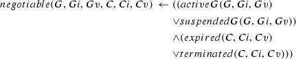
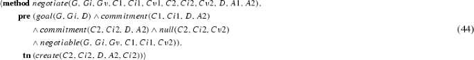
  • (g) $\frac{\langle G^{A \vee U},C^{E \vee T}\rangle }{\textsf {drop}(G)}\textsc {Abandon End Goal}$: If the end goal is active or suspended, and the commitment supporting that goal is expired or terminated, then drop the end goal.

    

• 2. Commitments to Means Goals: This item describes the rules relating a commitment $\mathsf {C}(x, y, s, u)$ in which agent y is the creditor to the means goal $G(y, s, f')$.

  • (a) $\frac{\langle G_2^N,C^C\rangle }{\textsf {consider}(G_2) \wedge \textsf {activate}(G_2)}\textsc {Detach}$: If the means goal is null, and the commitment is conditional, then consider the means goal.

  • (b) Detach’

    $\frac{\langle G_2^I,C^C\rangle }{\textsf {activate}(G_2)}\textsc {Detach'}$: If the means goal is inactive, and the commitment is conditional, then activate the means goal.

  • (c) Back Burner

    $\frac{\langle G_2^A,C^P\rangle }{\textsf {suspend}(G_2)}\textsc {Back Burner}$: If the means goal is active, and the commitment is pending, then suspend the means goal.

  • (d) Front Burner

    $\frac{\langle G_2^U,C^C\rangle }{\textsf {reactivate}(G_2)}\textsc {Front Burner}$: If the means goal is suspended, and the commitment is conditional, then reactivate the means goal.

  • (e) Abandon Means Goal

    $\frac{\langle G_2^A,C^{E \vee T}\rangle }{\textsf {drop}(G_2)}\textsc {Abandon Means Goal}$: If the means goal is active, and the commitment is expired or terminated, then drop the means goal.

  • (f) Persist

    $\frac{\langle G_2^{T \vee F},C^C\rangle }{\textsf {consider}(G'_2) \wedge \textsf {activate}(G'_2)}\textsc {Persist}$: If the means goal is terminated or failed, and the commitment is conditional, then consider an alternative means goal.

  • (g) Give Up

    $\frac{\langle G_2^{T \vee F},C^C\rangle }{\textsf {release}(C)}\textsc {Give Up}$: If the means goal is terminated or failed, and the commitment is conditional, then release the commitment.

• 3. Commitments to Discharge Goals: This item describes the rules relating a commitment $\mathsf {C}(x, y, s, u)$ in which agent x is the debtor to the discharge goal $G(x, u, f'')$.

  • (a) $\frac{\langle G_1^N,C^D\rangle }{\textsf {consider}(G_1) \wedge \textsf {activate}(G_1)}\textsc {Deliver}$: If the discharge goal is null, and the commitment is detached, then consider the discharge goal.

    

  • (b) $\frac{\langle G_1^N,C^D\rangle }{\textsf {activate}(G_1)}\textsc {Deliver'}$: If the discharge goal is inactive, and the commitment is detached, then activate the discharge goal.

    

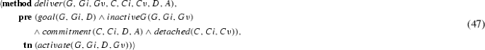
  • (c) $\frac{\langle G_1^A,C^P\rangle }{\textsf {suspend}(G_1)}\textsc {Back Burner}$: If the discharge goal is active, and the commitment is pending, then suspend the discharge goal.

    

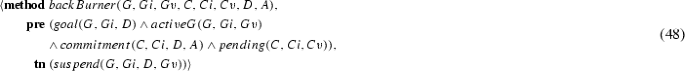
  • (d) $\frac{\langle G_1^U,C^D\rangle }{\textsf {reactivate}(G_1)}\textsc {Front Burner}$: If the discharge goal is suspended, and the commitment is detached, then reactivate the discharge goal.

    

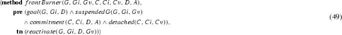
  • (e) $\frac{\langle G_1^A,C^{T \vee V}\rangle }{\textsf {drop}(G_1)}\textsc {Abandon Discharge Goal}$: If the discharge goal is active, and the commitment is terminated or violated, then drop the discharge goal.

    

  • (f) $\frac{\langle G_1^{T \vee F},C^D\rangle }{\textsf {consider}(G'_1) \wedge \textsf {activate}(G'_1)}\textsc {Persist}$: If the discharge goal is terminated or failed, and the commitment is detached, then consider an alternative discharge goal.

    

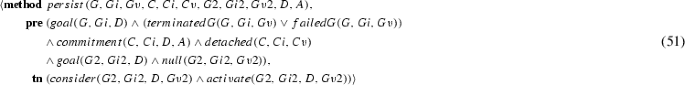
  • (g) $\frac{\langle G_1^{T \vee F},C^D\rangle }{\textsf {cancel}(C)}\textsc {Give Up}$: If the discharge goal is terminated or failed, and the commitment is detached, then cancel the commitment.

    

Appendix B: JSHOP domain-specific operators

Appendix C: JSHOP domain-specific methods

Appendix D: JSHOP methods for reasoning patterns

References

Alford, R., Bercher, P., & Aha, D. W. (2015). Tight bounds for HTN planning. In Proceedings of ICAPS’15 (pp. 7–15).
Apt, K. R. (1997). From logic programming to Prolog. Upper Saddle River, NJ: Prentice-Hall.
ASPE: The importance of radiology and pathology communication in the diagnosis and staging of cancer: Mammography as a case study (2010). Office of the Assistant Secretary for Planning and Evaluation, U.S. Department of Health and Human Services. http://aspe.hhs.gov/sp/reports/2010/PathRad/index.shtml.
Baldoni, M., Baroglio, C., Capuzzimati, F. & Micalizio, R. (2015). Exploiting social commitments in programming agent interaction. In Proceedings of PRIMA’15 (pp. 566–574).
Baldoni, M., Baroglio, C., Capuzzimati, F., & Micalizio, R. (2015). Leveraging commitments and goals in agent interaction. In Proceedings of 30th Italian conference on computational logic (CILC’15) (pp. 85–100).
Baldoni, M., Baroglio, C., Capuzzimati, F., & Micalizio, R. (2015). Programming with commitments and goals in JaCaMo+. In Proceedings of AAMAS’15 (pp. 1705–1706).
Baldoni, M., Baroglio, C., Chopra, A. K., & Singh, M. P. (2015). Composing and verifying commitment-based multiagent protocols. In Proceedings of IJCAI’15 (pp. 10–17).
Baldoni, M., Baroglio, C., Marengo, E., Patti, V., & Capuzzimati, F. (2014). Engineering commitment-based business protocols with the 2CL methodology. Autonomous Agents and Multi-Agent Systems, 28(4), 519–557.
Baldoni, M., Baroglio, C., & Micalizio, R. (2015). Social continual planning in open multiagent systems: A first study. In Proceedings of PRIMA’15 (pp. 575–584).
Barbulescu, L., Rubinstein, Z. B., Smith, S. F., & Zimmerman, T. L. (2010). Distributed coordination of mobile agent teams: The advantage of planning ahead. In Proceedings of AAMAS’10 (pp. 1331–1338) .
Bataineh, A. S., Bentahar, J., El-Menshawy, M., & Dssouli, R. (2017). Specifying and verifying contract-driven service compositions using commitments and model checking. Expert Systems with Applications, 74, 151–184.
Bellman, R. (1957). A markov decision process. Journal of Mathematical Mechanics, 6, 679–684.
Boddy, M., Horling, B., Phelps, J., Goldman, R., Vincent, R., Long, A., et al. (2007). c-TÆMS language specification. Technical report, Adventium Labs.
Bouguerra, A., & Karlsson, L. (2004). Hierarchical task planning under uncertainty. In 3rd Italian workshop on planning and scheduling (AI*IA’04), Perugia, Italy.
Brafman, R. I., & Domshlak, C. (2008). From one to many: Planning for loosely coupled multi-agent systems. In Proceedings of ICAPS’08 (pp. 28–35).
Castelfranchi, C. (1995). Commitments: From individual intentions to groups and organizations. In Proceedings of ICMAS’95 (pp. 41–48).
Chesani, F., Mello, P., Montali, M., & Torroni, P. (2013). Representing and monitoring social commitments using the event calculus. Autonomous Agents and Multi-Agent Systems, 27(1), 85–130.
Chopra, A. K., Dalpiaz, F., Aydemir, F. B., Giorgini, P., Mylopoulos, J., & Singh, M. P. (2014). Protos: Foundations for engineering innovative sociotechnical systems. In Proceedings of 22nd international requirements engineering conference (RE’14) (pp. 53–62).
Chopra, A. K., Dalpiaz, F., Giorgini, P., & Mylopoulos, J. (2010). Modeling and reasoning about service-oriented applications via goals and commitments. In Proceedings of 22nd international conference on advanced information systems engineering (CAiSE’10) (pp. 417–421).
Chopra, A. K., Dalpiaz, F., Giorgini, P., & Mylopoulos, J. (2010). Reasoning about agents and protocols via goals and commitments. In Proceedings of AAMAS’10 (pp. 457–464).
Chopra, A. K., & Singh, M. P. (2015). Cupid: Commitments in relational algebra. In Proceedings of 29th conference on artificial intelligence (AAAI’15) (pp. 2052–2059).
Chopra, A. K., & Singh, M. P. (2016). Custard: Computing norm states over information stores. In Proceedings of AAMAS’16 (pp. 1096–1105).
Chopra, A. K., & Singh, M. P. (2016). From social machines to social protocols: Software engineering foundations for sociotechnical systems. In Proceedings of WWW’16 (pp. 903–914).
Crosby, M., Jonsson, A., & Rovatsos, M. (2014). A single-agent approach to multiagent planning. In Proceedings of ECAI’14 (pp. 237–242).
Dastani, M., van der Torre, L., & Yorke-Smith, N. (2017). Commitments and interaction norms in organisations. Autonomous Agents and Multi-Agent Systems, 31(2), 207–249.
Della Penna, G., Intrigila, B., & Magazzeni, D. (2015). UPMurphi Released: PDDL+ Planning for hybrid systems. In Proceedings of 2nd ICAPS workshop on model checking and automated planning (pp. 35–39).
Desai, N., Chopra, A. K., & Singh, M. P. (2009). Amoeba: A methodology for modeling and evolution of cross-organizational business processes. ACM Transactions on Software Engineering and Methodology (TOSEM), 19(2), 6:1–6:45.
Durfee, E. (2001). Distributed problem solving and planning. In Multi-agent systems and applications, LNCS (Vol. 2086, pp. 118–149). Springer, New York, NY.
Erol, K., Hendler, J., & Nau, D. S. (1994). HTN planning: Complexity and expressivity. In Proceedings of AAAI’94 (Vol. 2, pp. 1123–1128).
Erol, K., Nau, D. S., & Subrahmanian, V. S. (1995). Complexity, decidability and undecidability results for domain-independent planning. Artificial Intelligence, 76(1–2), 75–88.
Fornara, N., & Colombetti, M. (2009). Ontology and time evolution of obligations and prohibitions using semantic web technology. In Declarative agent languages and technologies VII, LNCS (Vol. 5948, pp. 101–118). Springer, New York, NY.
Ghallab, M., Nau, D., & Traverso, P. (2004). Automated planning: Theory and practice. Burlington, MA: Elsevier.
Grosz, B. J., & Hunsberger, L. (2006). The dynamics of intention in collaborative activity. Cognitive Systems Research, 7(2–3), 259–272.
Guestrin, C., Koller, D., Parr, R., & Venkataraman, S. (2003). Efficient solution algorithms for factored MDPs. Journal of Artificial Intelligence Research, 19(10), 399–468.
Günay, A., Liu, Y., & Zhang, J. (2016). Promoca: Probabilistic modeling and analysis of agents in commitment protocols. Journal of Artificial Intelligence Research, 57, 465–508.
Günay, A., Winikoff, M., & Yolum, P. (2015). Dynamically generated commitment protocols in open systems. Autonomous Agents and Multi-Agent Systems, 29(2), 192–229.
Harland, J., Morley, D. N., Thangarajah, J., & Yorke-Smith, N. (2017). Aborting, suspending, and resuming goals and plans in BDI agents. Autonomous Agents and Multi-Agent Systems, 31(2), 288–331.
Hoffmann, J., Weber, I., & Kraft, F. M. (2010). SAP speaks PDDL. In Proceedings of AAAI’10.
Ilghami, O., & Nau, D. S. (2003). A general approach to synthesize problem-specific planners. Technical report, University of Maryland.
King, N. (2014). Expanding the boundaries of clinical informatics for interdisciplinary systems research. Health Systems, 3(1), 1–11.
Kun, C., Xu, J., & Reiff-Marganiec, S. (2009). Markov-HTN planning approach to enhance flexibility of automatic web service composition. In Proceedings of international conference on web services (ICWS’09) (pp. 9–16).
Kuter, U., Nau, D., Pistore, M., & Traverso, P. (2009). Task decomposition on abstract states, for planning under nondeterminism. Artificial Intelligence, 173(5–6), 669–695.
Kuter, U., & Nau, D. S. (2004). Forward-chaining planning in nondeterministic domains. In Proceedings of AAAI’04 (pp. 513–518).
Kuter, U., & Nau, D. S. (2005). Using domain-configurable search control for probabilistic planning. In Proceedings of AAAI’05 (pp. 1169–1174).
Lesser, V. R., Decker, K., Wagner, T., Carver, N., Garvey, A., Horling, B., et al. (2004). Evolution of the GPGP/TÆMS domain-independent coordination framework. Autonomous Agents and Multi-Agent Systems, 9(1–2), 87–143.
Maliah, S., Shani, G., & Stern, R. (2017). Collaborative privacy preserving multi-agent planning—Planners and heuristics. Autonomous Agents and Multi-Agent Systems, 31(3), 493–530.
Meneguzzi, F., Magnaguagno, M., Telang, P., Singh, M. P., & Yorke-Smith, N. (2017). meneguzzi/htn-goco: HTN goal commitment dynamics. https://doi.org/10.5281/zenodo.845435.
Meneguzzi, F., & de Silva, L. (2015). Planning in BDI agents: A survey of the integration of planning algorithms and agent reasoning. Knowledge Engineering Review, 30(1), 1–44.
Meneguzzi, F., Tang, Y., Sycara, K., & Parsons, S. (2011). An approach to generate MDPs using HTN representations. In Proceedings of IJCAI’11 workshop on decision making in partially observable, uncertain worlds.
Meneguzzi, F., Telang, P. R., & Singh, M. P. (2013). A first-order formalization of commitments and goals for planning. In Proceedings of AAAI’13 (pp. 1–8).
Meneguzzi, F., Telang, P. R., & Yorke-Smith, N. (2015). Towards planning uncertain commitment protocols. In Proceedings of AAMAS’15 (pp. 1681–1682).
Mouaddib, A. I., Boussard, M., & Bouzid, M. (2007). Towards a formal framework for multi-objective multiagent planning. In Proceedings of AAMAS’07.
Pistore, M., Marconi, A., Bertoli, P., & Traverso, P. (2005). Automated composition of web services by planning at the knowledge level. In Proceedings of IJCAI’05 (pp. 1252–1259).
Singh, M. P. (1991). Social and psychological commitments in multiagent systems. In AAAI fall symposium on knowledge and action at social and organizational levels (pp. 104–106).
Singh, M. P. (1999). An ontology for commitments in multiagent systems. AI and Law, 7, 97–113.
Singh, M. P. (2008). Semantical considerations on dialectical and practical commitments. In Proceedings of AAAI’08 (pp. 176–181).
Singh, M. P. (2012). Commitments in multiagent systems. In The goals of cognition: Essays in Honor of Cristiano Castelfranchi (pp. 601–626). College Publications, London, UK.
Singh, M. P. (2012). Norms as a basis for governing sociotechnical systems. ACM Transactions on Intelligent Systems and Technology (TIST), 5(1), 21:1–21:23.
Sohrabi, S., Baier, J. A., & McIlraith, S. A. (2009). HTN planning with preferences. In Proceedings of IJCAI’09 (pp. 1790 –1797).
Sultan, K., Bentahar, J., & El-Menshawy, M. (2014). Model checking probabilistic social commitments for intelligent agent communication. Applied Soft Computing, 22, 397–409.
Tang, Y., Meneguzzi, F., Sycara, K., & Parsons, S. (2011). Probabilistic hierarchical planning over MDPs. In Proceedings of AAMAS’11 (pp. 1143–1144).
Telang, P. R., Meneguzzi, F., & Singh, M. P. (2013). Hierarchical planning about goals and commitments. In Proceedings of AAMAS’13 (pp. 761–768).
Telang, P. R., Yorke-Smith, N., & Singh, M. P. (2012). Relating goal and commitment semantics. In Proceedings of 9th international workshop on programming multi-agent systems, LNCS (Vol. 7217, pp. 22–37). Springer, New York, NY.
Venkatraman, M., & Singh, M. P. (1999). Verifying compliance with commitment protocols. Autonomous Agents and Multi-Agent Systems, 2(3), 217–236.
Verdicchio, M., & Colombetti, M. (2002). Commitments for agent-based supply chain management. SIGecom Exchanges, 3(1), 13–23.
de Weerdt, M., & Clement, B. (2009). Introduction to planning in multiagent systems. Multiagent and Grid Systems, 5, 345–355.
Witwicki, S. J., & Durfee, E. H. (2007). Commitment-driven distributed joint policy search. In Proceedings of AAMAS’07 (pp. 492–499).
Xuan, P., & Lesser, V. R. (2000). Incorporating uncertainty in agent commitments. In Intelligent agents VI: Agent theories, architectures, and languages, LNCS (Vol. 1757, pp. 57–70). Springer, New York, NY.
Yolum, P., & Singh, M. P. (2002). Flexible protocol specification and execution: Applying event calculus planning using commitments. In Proceedings of AAMAS’02 (pp. 527–534).
Acknowledgements
We gratefully thank those who shared their code with us. Special thanks to Ugur Kuter. We thank the anonymous reviewers, and also acknowledge with gratitude the reviewers at ProMAS’11, AAMAS’13, AAAI’13, and AAMAS’15, where preliminary parts of this work appeared. FM thanks the Conselho Nacional de Desenvolvimento Científico e Tecnológico (CNPq) for the support within process numbers 306864/2013-4 under the PQ fellowship and 482156/2013-9 under the Universal project programs. NYS acknowledges support of the AUB University Research Board Grant Number 102853 and the OSB Grant OFFER_C1_2013_2014.
Author information
Authors and Affiliations
Corresponding author