Log in

Planning step-stress test plans under Type-I hybrid censoring for the log-location-scale distribution

  • Original Paper
  • Published:
Statistical Methods & Applications Aims and scope Submit manuscript

Abstract

The optimal design of a k-level step-stress accelerated life-testing (ALT) experiment with unequal duration steps under Type-I hybrid censoring scheme for a general log-location-scale lifetime distribution is discussed here. Censoring is allowed only at the change-stress point in the final stage. Based on the cumulative exposure model, the determination of the optimal choice for Weibull, lognormal and log-logistic lifetime distributions are considered by minimization of the asymptotic variance of the maximum likelihood estimate of the pth percentile of the lifetime at the normal operating condition. Numerical results show that for these lifetime distributions, the optimal k-step-stress ALT design with unequal duration steps under Type-I hybrid censoring scheme reduces just to a 2-step-stress ALT design.

This is a preview of subscription content, log in via an institution to check access.

Access this article

Price excludes VAT (USA)
Tax calculation will be finalised during checkout.

Instant access to the full article PDF.

Institutional subscriptions

References

  • Alhadeed AA, Yang SS (2005) Optimal simple step-stress plan for cumulative exposure model using log-normal distribution. IEEE Trans Reliab 54:64–68

    Article  Google Scholar 

  • Bai DS, Kim MS (1993) Optimum simple step-stress accelerated life tests for Weibull distribution and Type I censoring. Naval Res Logist 40:193–210

    Article  Google Scholar 

  • Bai DS, Kim MS, Lee SH (1989) Optimum simple step-stress accelerated life test with censoring. IEEE Trans Reliab 38:528–532

    Article  Google Scholar 

  • Balakrishnan N (2009) A synthesis of exact inferential results for exponential step-stress models and associated optimal accelerated life-tests. Metrika 69:351–396

    Article  MathSciNet  Google Scholar 

  • Balakrishnan N, Han D (2009) Optimal step-stress testing for progressively Type-I censored data from exponential distribution. J Stat Plan Inference 139:1782–1798

    Article  MathSciNet  Google Scholar 

  • Balakrishnan N, Kundu D (2013) Hybrid censoring: models, inferential results and applications. Comput Stat Data Anal 57:166–209 (with discussions)

    Article  MathSciNet  Google Scholar 

  • Balakrishnan N, Xie Q (2007) Exact inference for a simple step-stress model with Type-I hybrid censored data from the exponential distribution. J Stat Plan Inference 137:3268–3290

    Article  MathSciNet  Google Scholar 

  • Balakrishnan N, Zhang L, Xie Q (2009) Inference for a simple step-stress model with Type-I censoring and lognormally distributed lifetimes. Commun Stat Theory Methods 38:1690–1709

    Article  MathSciNet  Google Scholar 

  • Chung SW, Bai DS (1998) Optimal designs of simple step-stress accelerated life tests for lognormal lifetime distributions. Int J Reliab Qual Saf Eng 5:315–336

    Article  Google Scholar 

  • Chung SW, Seo YS, Yun WY (2006) Acceptance sampling plans based on failure-censored step-stress accelerated tests for Weibull distributions. J Qual Maint Eng 12:373–396

    Article  Google Scholar 

  • Corana A, Marchesi M, Martini C, Ridella S (1987) Minimizing multi-modal functions of continuous variables with the “simulated annealing” algorithm. ACM Trans Math Softw 13:262–280

    Article  Google Scholar 

  • Dharmadhikari AD, Rahman MM (2003) A model for step-stress accelerated life testing. Naval Res Logist 50:841–868

    Article  MathSciNet  Google Scholar 

  • Ding C, Yang C, Tse S-K (2010) Accelerated life test sampling plans for the Weibull distribution under Type I progressive interval censoring with random removals. J Stat Comput Simul 80:903–914

    Article  MathSciNet  Google Scholar 

  • Fard N, Li C (2009) Optimal simple step stress accelerated life test design for reliability prediction. J Stat Plan Inference 139:1799–1808

    Article  MathSciNet  Google Scholar 

  • Gouno E, Sen A, Balakrishnan N (2004) Optimal step-stress test under progressive Type-I censoring. IEEE Trans Reliab 53:383–393

    Article  Google Scholar 

  • Han D, Balakrishnan N, Sen A, Gouno E (2006) Corrections on “Optimal step-stress test under progressive Type-I censoring”. IEEE Trans Reliab 55:613–614

    Article  Google Scholar 

  • Jones MC, Noufaily A (2015) Log-location-scale-log-concave distributions for survival and reliability analysis. Electron J Stat 9:2732–2750

    Article  MathSciNet  Google Scholar 

  • Kateri M, Balakrishnan N (2008) Inference for a simple step-stress model with Type-II censoring, and Weibull distributed lifetimes. IEEE Trans Reliab 57:616–626

    Article  Google Scholar 

  • Khamis IH (1997) Optimum \(m\)-step, step-stress design with \(k\) stress variables. Commun Stat Simul Comput 26:1301–1313

    Article  Google Scholar 

  • Khamis IH, Higgins JJ (1996) Optimum 3-step step-stress tests. IEEE Trans Reliab 45:341–345

    Article  Google Scholar 

  • Kiefer J (1974) General equivalence theory for optimum designs (approximate theory). Ann Stat 2:849–879

    Article  MathSciNet  Google Scholar 

  • Lin CT, Chou CC, Balakrishnan N (2013) Planning step-stress test plans under Type-I censoring for the log-location-scale case. J Stat Comput Simul 83:1852–1867

    Article  MathSciNet  Google Scholar 

  • Lin CT, Chou CC, Balakrishnan N (2014) Planning step-stress test under Type-I censoring for the exponential case. J Stat Comput Simul 84:819–832

    Article  MathSciNet  Google Scholar 

  • Lin CT, Huang YL, Balakrishnan N (2011) Exact Bayesian variable sampling plans for the exponential distribution with progressive hybrid censoring. J Stat Comput Simul 81:873–882

    Article  MathSciNet  Google Scholar 

  • Ling L, Xu W, Li M (2011) Optimal bivariate step-stress accelerated life test for Type-I hybrid censored data. J Stat Comput Simul 81:1175–1186

    Article  MathSciNet  Google Scholar 

  • Ma H, Meeker WQ (2008) Optimum step-stress accelerated life test plans for log-location-scale distributions. Naval Res Logist 55:551–562

    Article  MathSciNet  Google Scholar 

  • Miller R, Nelson WB (1983) Optimum simple step-stress plans for accelerated life testing. IEEE Trans Reliab 32:59–65

    Article  Google Scholar 

  • Nelson WB (1990) Accelerated testing: statistical models, test plans, and data analysis. Wiley, New York

    Book  Google Scholar 

  • Nelson WB (2005a) A bibliography of accelerated test plans, part I-overview. IEEE Trans Reliab 54:194–197

    Article  Google Scholar 

  • Nelson WB (2005b) A bibliography of accelerated test plans, part II-references. IEEE Trans Reliab 54:370–373

    Article  Google Scholar 

  • Nelson WB, Kielpinski TJ (1976) Theory for optimum censored accelerated life tests for normal and lognormal life distributions. Technometrics 18:105–114

    Article  Google Scholar 

  • Srivastava PW, Shukla R (2008) A log-logistic step-stress model. IEEE Trans Reliab 57:431–434

    Article  Google Scholar 

  • Tang LC, Sun YS, Goh TN, Ong HL (1996) Analysis of step-stress accelerated-life-test data: a new approach. IEEE Trans Reliab 45:69–74

    Article  Google Scholar 

  • Wu SJ, Lin YP, Chen YJ (2006) Planning step-stress life test with progressively Type-I group-censored exponential data. Stat Neerl 60:46–56

    Article  MathSciNet  Google Scholar 

  • Wu SJ, Lin YP, Chen ST (2008) Optimal step-stress test under Type-I progressive group-censoring with random removals. J Stat Plan Inference 138:817–826

    Article  MathSciNet  Google Scholar 

  • Yeo KP, Tang LC (1999) Planning step-stress life-test with a target acceleration-factor. IEEE Trans Reliab 54:370–373

    Google Scholar 

Download references

Acknowledgements

The authors express their sincere thanks to the Editor, Associate Editor, and an anonymous reviewer for their valuable comments and suggestions on an earlier version of this manuscript which led to this improved version. The first author thanks the Ministry of Science and Technology of the Republic of China, Taiwan (Contract No: MOST 106-2118-M-032-006-MY2) for funding this research.

Author information

Authors and Affiliations

Authors

Corresponding author

Correspondence to Chien-Tai Lin.

Additional information

Publisher's Note

Springer Nature remains neutral with regard to jurisdictional claims in published maps and institutional affiliations.

Appendix

Appendix

For deriving the entries of the Fisher information matrix, we need the following properties concerning the count variables and order statistics.

Some important properties

  1. (a)

    The random variable \(n_1\) has a binomial distribution with parameters \((n, \Phi (\eta _1))\). For \(i=2, 3, \ldots , k-1\), given \(n_1, n_2, \ldots , n_{i-1}\), the random variable \(n_i\) has a binomial distribution with parameters \( \displaystyle \left( n-\sum _{j=1}^{i-1} n_j, \frac{\Phi (\eta _i)-\Phi (\eta _{i-1})}{1- \Phi (\eta _{i-1})} \right) \); here,

    $$\begin{aligned} \eta _i=\frac{\ln (\tau _i+ s_{i-1}- \tau _{i-1})- (\beta _0+ \beta _1 x_i)}{\sigma }, \quad i=1, 2, \ldots , k, \ \eta _0 \equiv -\infty ; \end{aligned}$$
    (4)
  2. (b)

    Given \(n_1, n_2, \ldots , n_{k-1}\), the random variable \(n_k^*\) has probability mass function
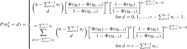
  3. (c)

    Given \(n_1, n_2, \ldots , n_i\), the random variables \(y_{i,j}\), \(j=1, 2, \ldots , n_i\), are distributed jointly as order statistics from a random sample of size \(n_i\) from a doubly truncated population with PDF \( \displaystyle \frac{g_i(y)}{\Phi (\eta _{i})-\Phi (\eta _{i-1})}\) for \( \tau _{i-1} \le y \le \tau _i\) and \(i=1, 2, \ldots , k-1\), where \(g_i(\cdot )\) is as defined earlier in (2);

  4. (d)

    Given \(n_1, n_2, \ldots , n_{k-1}\), the random variables \(y_{k,j}\), \(j=1, 2, \ldots , n_k^*\), are distributed jointly as order statistics from a random sample of size \(n_k^*\) from a doubly truncated population with PDF \(\displaystyle \frac{g_k(y)}{\Phi (\eta _{k})-\Phi (\eta _{k-1})}\) for \(\tau _{k-1} < y \le \tau _k\).

Using the above key distributional properties, we obtain

$$\begin{aligned}&E(n_i)= n [ \Phi (\eta _i)- \Phi (\eta _{i-1})], \\&E\left\{ \frac{Z^{\ell }_i e^{-q \sigma Z_i}}{\phi (Z_i)} \left[ \frac{1}{\phi (Z_i)} \left( \frac{d \phi (Z_i)}{d Z_i}\right) ^2- \frac{d^2 \phi (Z_i)}{d Z_i^2} \right] \right\} = \frac{A_{i, q,{\ell }}}{\Phi (\eta _{i})-\Phi (\eta _{i-1})}, \\&E\left( \frac{Z^{\ell }_i e^{-q \sigma Z_i}}{\phi (Z_i)} \frac{d \phi (Z_i)}{d Z_i} \right) = \frac{B_{i, q, {\ell }}}{\Phi (\eta _{i})-\Phi (\eta _{i-1})}, \\&E\left( e^{-q \sigma Z_i} \right) = \frac{C_{i,q}}{\Phi (\eta _{i})-\Phi (\eta _{i-1})} , \end{aligned}$$

for \(q=0, 1, 2, \ell =0, 1, 2\), and \(i=1, \ldots , k\), where

$$\begin{aligned} A_{i, q, {\ell }}= & {} \int _{\eta _{i-1}}^{\eta _{i}} z^{\ell } e^{-q \sigma z} \left[ \frac{1}{\phi (z)} \left( \frac{d \phi (z)}{d z}\right) ^2- \frac{d^2 \phi (z)}{d z^2}\right] dz,\\ B_{i, q, {\ell }}= & {} \int _{\eta _{i-1}}^{\eta _{i}} z^{\ell } e^{-q \sigma z} \frac{d \phi (z)}{d z} dz,\\ C_{i,q}= & {} \int _{\eta _{i-1}}^{\eta _{i}} e^{-q \sigma z} \phi (z) dz. \end{aligned}$$

For \(q=0, 1, 2\), \(\ell =0, 1, 2\), and \(h=0,1\), we define

$$\begin{aligned} A^*_{q, {\ell }}= & {} \frac{1}{n} E\left\{ \sum _{j=1}^{n^*_k} \frac{Z_k^{\ell } e^{-q \sigma Z_k}}{\phi (Z_k)} \left[ \frac{1}{\phi (Z_k)} \left( \frac{d \phi (Z_k)}{d Z_k}\right) ^2- \frac{d^2 \phi (Z_k)}{d Z_k^2} \right] \right\} ,\\ B^*_{q, {\ell }}= & {} \frac{1}{n} E\left( \sum _{j=1}^{n^*_k} \frac{Z_k^{\ell } e^{-q \sigma Z_k}}{\phi (Z_k)} \frac{d \phi (Z_k)}{d Z_k} \right) ,\\ C^*_{q}= & {} \frac{1}{n} E\left( \sum _{j=1}^{n^*_k} e^{-q \sigma Z_k} \right) ,\\ D^*_{q, {\ell }, h}= & {} \frac{1}{n} E \left[ \left( n- \sum _{i=1}^{k-1} n_i -n^*_k\right) \frac{{\eta _k^*}^{\ell } \phi ^h (\eta _k^*) e^{-q \sigma \eta _k^*}}{1-\Phi (\eta ^*_k)} \right] ,\\ H^*_{q,{\ell }}= & {} \frac{1}{n} E \left\{ \left( n- \sum _{i=1}^{k-1} n_i -n^*_k\right) \frac{{\eta _k^*}^{\ell } e^{-q \sigma \eta _k^*}}{1-\Phi (\eta ^*_k)} \left[ \frac{d \phi (\eta _k^*)}{d \eta _k^*}+ \frac{\phi ^2 (\eta _k^*)}{1-\Phi (\eta _k^*)} \right] \right\} . \end{aligned}$$

We then have

$$\begin{aligned} A^*_{q, {\ell }}= & {} \frac{1}{n} E\left\{ \sum _{j=1}^{n^*_k} \frac{Z_k^{\ell } e^{-q \sigma Z_k}}{\phi (Z_k)} \left[ \frac{1}{\phi (Z_k)} \left( \frac{d \phi (Z_k)}{d Z_k} \right) ^2- \frac{d^2 \phi (Z_k)}{d Z_k^2} \right] \right\} \\= & {} \frac{1}{n} E\left\{ E(n^*_k) E \left\{ \frac{Z_k^{\ell } e^{-q \sigma Z_k}}{\phi (Z_k)} \left[ \frac{1}{\phi (Z_k)} \left( \frac{d \phi (Z_k)}{d Z_k} \right) ^2- \frac{d^2 \phi (Z_k)}{d Z_k^2} \right] \right\} \bigg | \tau _k^* \right\} \\= & {} \frac{1}{n} E\left\{ E(n^*_k) E\left\{ \frac{Z_k^{\ell } e^{-q \sigma Z_k}}{\phi (Z_k)} \left[ \frac{1}{\phi (Z_k)} \left( \frac{d \phi (Z_k)}{d Z_k} \right) ^2- \frac{d^2 \phi (Z_k)}{d Z_k^2} \right] \right\} \bigg | Y_{r:n}> \tau _k \right\} \\&\times \, P(Y_{r:n}> \tau _k)\\&+\ \frac{1}{n} E\left\{ E(n^*_k) E\left\{ \frac{Z_k^{\ell } e^{-q \sigma Z_k}}{\phi (Z_k)} \left[ \frac{1}{\phi (Z_k)} \left( \frac{d \phi (Z_k)}{d Z_k} \right) ^2- \frac{d^2 \phi (Z_k)}{d Z_k^2} \right] \right\} \bigg | \tau _{k-1}< Y_{r:n}< \tau _k \right\} \\&\times P(\tau _{k-1}< Y_{r:n}< \tau _k)\\= & {} \frac{1}{n} E(n_k) E\left\{ \frac{Z_k^{\ell } e^{-q \sigma Z_k}}{\phi (Z_k)} \left[ \frac{1}{\phi (Z_k)} \left( \frac{d \phi (Z_k)}{d Z_k} \right) ^2- \frac{d^2 \phi (Z_k)}{d Z_k^2} \right] \right\} P(Y_{r:n}> \tau _k)\\&+\ \frac{1}{n} E\left\{ n \left[ \Phi \left( Z_{k, r-\sum _{i=1}^{k-1} n_i}\right) - \Phi (\eta _{k-1})\right] \right. \\&\left. \times \int _{\eta _{k-1}}^{Z_{k, r-\sum _{i=1}^{k-1} n_i}} \frac{x^{\ell } e^{-q \sigma x}}{\phi (x)} \left[ \frac{1}{\phi (x)} \left( \frac{d \phi (x)}{d x} \right) ^2- \frac{d^2 \phi (x)}{d x^2} \right] \right. \\&\times \left. \frac{\phi (x)}{\Phi \left( Z_{k, r-\sum _{i=1}^{k-1} n_i}\right) - \Phi (\eta _{k-1})} \ dx \bigg | \tau _{k-1}< Y_{r:n}< \tau _k \right\} P(\tau _{k-1}< Y_{r:n}< \tau _k)\\= & {} A_{k, q, \ell } P(Y_{r:n}> \tau _k)\\&+\ E \left\{ \int _{\eta _{k-1}}^{Z_{k, r-\sum _{i=1}^{k-1} n_i}} x^{\ell } e^{-q \sigma x} \left[ \frac{1}{\phi (x)} \left( \frac{d \phi (x)}{d x} \right) ^2- \frac{d^2 \phi (x)}{d x^2} \right] \ dx \bigg | \tau _{k-1}< Y_{r:n}< \tau _k \right\} \\&\times P(\tau _{k-1}< Y_{r:n} < \tau _k)\\= & {} A_{k, q, \ell } P(Y_{r:n}> \tau _k) +\left[ r-\sum _{i=1}^{k-1} E(n_i) \right] {n-\sum _{i=1}^{k-1} E(n_i) \atopwithdelims ()r-\sum _{i=1}^{k-1} E(n_i)}\\&\times \int ^{\tau _k}_{\tau _{k-1}} \left\{ \int _{\eta _{k-1}}^{z_{k, r-\sum _{i=1}^{k-1} n_i}} x^{\ell } e^{-q \sigma x} \left[ \frac{1}{\phi (x)} \left( \frac{d \phi (x)}{d x} \right) ^2- \frac{d^2 \phi (x)}{d x^2} \right] \ dx \right\} \\&\times \left[ \frac{G_k (y)-G_{k-1} (\tau _{k-1})}{1-G_{k-1} (\tau _{k-1})}\right] ^{r-\sum _{i=1}^{k-1} E(n_i)-1} \left[ \frac{1-G_k (y)}{1-G_{k-1} (\tau _{k-1})}\right] ^{n-r} \frac{g_k (y)}{1-G_{k-1} (\tau _{k-1})} \ dy\\= & {} A_{k, q, \ell } P(Y_{r:n}> \tau _k) +\left[ r-\sum _{i=1}^{k-1} E(n_i) \right] {n-\sum _{i=1}^{k-1} E(n_i) \atopwithdelims ()r-\sum _{i=1}^{k-1} E(n_i)} \\&\times \int ^{\eta _k}_{\eta _{k-1}} \left\{ \int _{\eta _{k-1}}^{w} x^{\ell } e^{-q \sigma x} \left[ \frac{1}{\phi (x)} \left( \frac{d \phi (x)}{d x} \right) ^2- \frac{d^2 \phi (x)}{d x^2} \right] \ dx \right\} \\&\times \left[ \frac{\Phi (w)-\Phi (\eta _{k-1})}{1-\Phi (\eta _{k-1})}\right] ^{r-\sum _{i=1}^{k-1} E(n_i)-1} \left[ \frac{1-\Phi (w)}{1-\Phi (\eta _{k-1})}\right] ^{n-r} \frac{\phi (w)}{1-\Phi (\eta _{k-1})} \ dw,\\ B^*_{q, {\ell }}= & {} B_{k, q, \ell } P(Y_{r:n}> \tau _k)\\&+\left[ r-\sum _{i=1}^{k-1} E(n_i) \right] {n-\sum _{i=1}^{k-1} E(n_i) \atopwithdelims ()r-\sum _{i=1}^{k-1} E(n_i)} \int ^{\eta _k}_{\eta _{k-1}} \left\{ \int _{\eta _{k-1}}^{w} x^{\ell } e^{-q \sigma x} \frac{d \phi (x)}{d x} \ dx \right\} \\&\times \left[ \frac{\Phi (w)-\Phi (\eta _{k-1})}{1-\Phi (\eta _{k-1})}\right] ^{r-\sum _{i=1}^{k-1} E(n_i)-1} \left[ \frac{1-\Phi (w)}{1-\Phi (\eta _{k-1})}\right] ^{n-r} \frac{\phi (w)}{1-\Phi (\eta _{k-1})} \ dw,\\ C^*_{q}= & {} C_{k, q} P(Y_{r:n} > \tau _k)\\&+\left[ r-\sum _{i=1}^{k-1} E(n_i) \right] {n-\sum _{i=1}^{k-1} E(n_i) \atopwithdelims ()r-\sum _{i=1}^{k-1} E(n_i)} \int ^{\eta _k}_{\eta _{k-1}} \left\{ \int _{\eta _{k-1}}^{w} e^{-q \sigma x} \phi (x) \ dx \right\} \\&\times \left[ \frac{\Phi (w)-\Phi (\eta _{k-1})}{1-\Phi (\eta _{k-1})}\right] ^{r-\sum _{i=1}^{k-1} E(n_i)-1} \left[ \frac{1-\Phi (w)}{1-\Phi (\eta _{k-1})}\right] ^{n-r} \frac{\phi (w)}{1-\Phi (\eta _{k-1})} \ dw, \end{aligned}$$

and

$$\begin{aligned} D^*_{q, {\ell }, h}= & {} \frac{1}{n} E \left[ \left( n- \sum _{i=1}^{k-1} n_i -n^*_k\right) \frac{{\eta _k^*}^{\ell } \phi ^h (\eta _k^*) e^{-q \sigma \eta _k^*}}{1-\Phi (\eta ^*_k)} \right] \\= & {} \frac{1}{n} E\left[ \left( n- \sum _{i=1}^{k-1} E(n_i) -E(n^*_k) \right) E \left( \frac{{\eta _k^*}^{\ell } \phi ^h (\eta _k^*) e^{-q \sigma \eta _k^*}}{1-\Phi (\eta ^*_k)} \right) \bigg | \tau _k^* \right] \\= & {} \frac{1}{n} E\left[ \left( n- \sum _{i=1}^{k-1} E(n_i) -E(n^*_k) \right) E \left( \frac{{\eta _k^*}^{\ell } \phi ^h (\eta _k^*) e^{-q \sigma \eta _k^*}}{1-\Phi (\eta ^*_k)} \right) \bigg | Y_{r:n}> \tau _k \right] P(Y_{r:n}> \tau _k)\\&+\ \frac{1}{n} E\left[ \left( n- \sum _{i=1}^{k-1} E(n_i) -E(n^*_k) \right) E \left( \frac{{\eta _k^*}^{\ell } \phi ^h (\eta _k^*) e^{-q \sigma \eta _k^*}}{1-\Phi (\eta ^*_k)} \right) \bigg | \tau _{k-1}< Y_{r:n}< \tau _k \right] \\&\times P(\tau _{k-1}< Y_{r:n}< \tau _k)\\= & {} \frac{1}{n} \left( n- \sum _{i=1}^{k-1} E(n_i) -E(n_k) \right) \frac{{\eta _k}^{\ell } \phi ^h (\eta _k) e^{-q \sigma \eta _k}}{1-\Phi (\eta _k)} P(Y_{r:n}> \tau _k)\\&+\ \frac{1}{n} E\left\{ \left\{ n- \sum _{i=1}^{k-1} n [ \Phi (\eta _i)- \Phi (\eta _{i-1})] -n \left[ \Phi \left( Z_{k, r-\sum _{i=1}^{k-1} n_i}\right) - \Phi (\eta _{k-1})\right] \right\} \right. \\&\times \frac{Z_{k, r-\sum _{i=1}^{k-1} n_i}^{\ell } \phi ^h (Z_{k, r-\sum _{i=1}^{k-1} n_i}) e^{-q \sigma Z_{k, r-\sum _{i=1}^{k-1} n_i}}}{1-\Phi (Z_{k, r-\sum _{i=1}^{k-1} n_i})} \bigg | \tau _{k-1}< Y_{r:n}< \tau _k \Bigg \} P(\tau _{k-1}< Y_{r:n} < \tau _k)\\= & {} {\eta _k}^{\ell } \phi ^h (\eta _k) e^{-q \sigma \eta _k} P(Y_{r:n}> \tau _k) +\left[ r-\sum _{i=1}^{k-1} E(n_i) \right] {n-\sum _{i=1}^{k-1} E(n_i) \atopwithdelims ()r-\sum _{i=1}^{k-1} E(n_i)}\\&\times \int ^{\tau _k}_{\tau _{k-1}} z_{k, r-\sum _{i=1}^{k-1} n_i}^{\ell } \phi ^h (z_{k, r-\sum _{i=1}^{k-1} n_i}) e^{-q \sigma z_{k, r-\sum _{i=1}^{k-1} n_i}}\\&\times \left[ \frac{G_k (y)-G_{k-1} (\tau _{k-1})}{1-G_{k-1} (\tau _{k-1})}\right] ^{r-\sum _{i=1}^{k-1} E(n_i)-1} \left[ \frac{1-G_k (y)}{1-G_{k-1} (\tau _{k-1})}\right] ^{n-r} \frac{g_k (y)}{1-G_{k-1} (\tau _{k-1})} \ dy\\= & {} {\eta _k}^{\ell } \phi ^h (\eta _k) e^{-q \sigma \eta _k} P(Y_{r:n}> \tau _k)\\&+\left[ r-\sum _{i=1}^{k-1} E(n_i) \right] {n-\sum _{i=1}^{k-1} E(n_i) \atopwithdelims ()r-\sum _{i=1}^{k-1} E(n_i)} \int ^{\eta _k}_{\eta _{k-1}} w^{\ell } \phi ^{h} (w) e^{-q \sigma w}\\&\times \left[ \frac{\Phi (w)-\Phi (\eta _{k-1})}{1-\Phi (\eta _{k-1})}\right] ^{r-\sum _{i=1}^{k-1} E(n_i)-1} \left[ \frac{1-\Phi (w)}{1-\Phi (\eta _{k-1})}\right] ^{n-r} \frac{\phi (w)}{1-\Phi (\eta _{k-1})} \ dw,\\ H^*_{q, {\ell }}= & {} {\eta _k}^{\ell } e^{-q \sigma \eta _k} \left[ \frac{d \phi (\eta _k)}{d \eta _k}+ \frac{\phi ^2 (\eta _k)}{1-\Phi (\eta _k)} \right] P(Y_{r:n} > \tau _k)\\&+\left[ r-\sum _{i=1}^{k-1} E(n_i) \right] {n-\sum _{i=1}^{k-1} E(n_i) \atopwithdelims ()r-\sum _{i=1}^{k-1} E(n_i)} \int ^{\eta _k}_{\eta _{k-1}} w^{\ell } e^{-q \sigma w} \left[ \frac{d \phi (w)}{d w}+ \frac{\phi ^2 (w)}{1-\Phi (w)} \right] \\&\times \left[ \frac{\Phi (w)-\Phi (\eta _{k-1})}{1-\Phi (\eta _{k-1})}\right] ^{r-\sum _{i=1}^{k-1} E(n_i)-1} \left[ \frac{1-\Phi (w)}{1-\Phi (\eta _{k-1})}\right] ^{n-r} \frac{\phi (w)}{1-\Phi (\eta _{k-1})} \ dw, \end{aligned}$$

and

$$\begin{aligned} P(Y_{r:n} > \tau _k)= & {} \bigg [ r-\sum _{i=1}^{k-1} E(n_i) \bigg ] {n-\sum _{i=1}^{k-1} E(n_i) \atopwithdelims ()r-\sum _{i=1}^{k-1} E(n_i)}\int ^{\infty }_{\eta _k} \left[ \frac{\Phi (w)-\Phi (\eta _{k-1})}{1-\Phi (\eta _{k-1})}\right] ^{r-\sum _{i=1}^{k-1} E(n_i)-1} \\&\times \left[ \frac{1-\Phi (w)}{1-\Phi (\eta _{k-1})}\right] ^{n-r} \frac{\phi (w)}{1-\Phi (\eta _{k-1})} \ dw. \end{aligned}$$

Hence, the entries of the Fisher information matrix are as follows:

$$\begin{aligned} I_{11}= & {} \frac{n}{\sigma ^2} \left\{ \sum _{i=1}^{k-1} A_{i,0,0}+ A^*_{0,0}+ H^*_{0,0} \right\} ,\\ I_{12}= & {} \frac{n}{\sigma ^2} \left\{ \sum _{i=1}^{k-1} x_i A_{i,0,0}+ x_k A^*_{0,0} -\sum _{i=2}^{k-1} A_{i,1,0} \sum _{h=2}^{i} (x_{h} -x_{h-1}) s_{h-1} e^{-\mu _h} \right. \\&\left. -\ A^*_{1,0} \sum _{h=2}^{k} (x_{h} -x_{h-1}) s_{h-1} e^{-\mu _h} + x_k H^*_{0,0}{-} H^*_{1,0} \sum _{h=2}^{k} (x_{h} - x_{h-1}) s_{h-1} e^{-\mu _h} \right\} \!,\\ I_{13}= & {} \frac{n}{\sigma ^2} \left\{ \sum _{i=1}^{k-1} A_{i,0,1}+ A^*_{0,1}+ H^*_{0,1} \right\} ,\\ I_{22}= & {} \frac{n}{\sigma ^2} \left\{ \sum _{i=1}^{k-1} x_i^2 A_{i,0,0} +x_k^2 A^*_{0,0} -2 \sum _{i=2}^{k-1} x_i A_{i,1,0} \sum _{h=2}^{i} (x_{h} -x_{h-1}) s_{h-1} e^{-\mu _h} \right. \\&-\ 2 x_k A^*_{1,0} \sum _{h=2}^{k} (x_{h} -x_{h-1}) s_{h-1} e^{-\mu _h}\\&+\ \sum _{i=2}^{k-1} A_{i,2,0} \left[ \sum _{h=2}^{i} (x_{h} -x_{h-1}) s_{h-1} e^{-\mu _h}\right] ^2\\&+A^*_{2,0} \left[ \sum _{h=2}^{k} (x_{h} -x_{h-1}) s_{h-1} e^{-\mu _h}\right] ^2\\&-\ \sigma \sum _{i=2}^{k-1} (B_{i,1,0}- \sigma C_{i,1}) \sum _{h=2}^{i} \sum _{\ell =2}^{h} (x_{h} -x_{h-1}) (x_{\ell } -x_{\ell -1}) s_{\ell -1} e^{ -\mu _\ell }\\&-\ \sigma (B^*_{1,0}- \sigma C^*_{1}- D^*_{1,0,1}) \sum _{h=2}^{k} \sum _{\ell =2}^{h} (x_{h} -x_{h-1}) (x_{\ell } -x_{\ell -1}) s_{\ell -1} e^{ -\mu _\ell }\\&-\ \sigma \sum _{i=2}^{k-1} (B_{i,1,0}- \sigma C_{i,1}) \sum _{h=2}^{i} (x_{h} -x_{h-1}) (x_{i} -x_{h}) s_{h-1} e^{ -\mu _h}\\&-\ \sigma (B^*_{1,0}- \sigma C^*_{1}- D^*_{1,0,1}) \sum _{h=2}^{k} (x_{h} -x_{h-1}) (x_{k} -x_{h}) s_{h-1} e^{ -\mu _h}\\&+\ \sigma \sum _{i=2}^{k-1} (B_{i,2,0}- \sigma C_{i,2}) \left[ \sum _{h=2}^{i} (x_{h} -x_{h-1}) s_{h-1} e^{ -\mu _h} \right] ^2\\&+\ \sigma (B^*_{2,0}- \sigma C^*_{2}- D^*_{2,0,1}) \left[ \sum _{h=2}^{k} (x_{h} -x_{h-1}) s_{h-1} e^{ -\mu _h} \right] ^2\\&+\ x_k^2 H^*_{0,0} -2x_k H^*_{1,0} \sum _{h=2}^{k} (x_{h} -x_{h-1}) s_{h-1} e^{-\mu _{h}}\\&\left. +H^*_{2,0} \left[ \sum _{h=2}^{k} (x_{h} -x_{h-1}) s_{h-1} e^{-\mu _{h}}\right] ^2 \right\} ,\\ I_{23}= & {} \frac{n}{\sigma ^2} \left\{ \sum _{i=1}^{k-1} x_i A_{i,0,1} +x_k A^*_{0,1} -\sum _{i=2}^{k-1} (A_{i,1,1}- \sigma C_{i,1}) \sum _{h=2}^{i} (x_{h} -x_{h-1}) s_{h-1} e^{-\mu _h} \right. \\&-\ (A^*_{1,1}- \sigma C^*_{1}) \sum _{h=2}^{k} (x_{h} -x_{h-1}) s_{h-1} e^{-\mu _h} +x_k H^*_{0,1}\\&\left. - H^*_{1,1} \sum _{h=2}^{k} (x_{h} -x_{h-1}) s_{h-1} e^{-\mu _{h}} \right\} ,\\ \text{ and } \\ I_{33}= & {} \frac{n}{\sigma ^2} \left\{ \sum _{i=1}^{k-1} (A_{i,0,2}-B_{i,0,1})+ A^*_{0,2}- B^*_{0,1}+ D^*_{0,1,1}+ H^*_{0,2} \right\} . \end{aligned}$$

Rights and permissions

Reprints and permissions

About this article

Check for updates. Verify currency and authenticity via CrossMark

Cite this article

Lin, CT., Chou, CC. & Balakrishnan, N. Planning step-stress test plans under Type-I hybrid censoring for the log-location-scale distribution. Stat Methods Appl 29, 265–288 (2020). https://doi.org/10.1007/s10260-019-00476-8

Download citation

  • Accepted:

  • Published:

  • Issue Date:

  • DOI: https://doi.org/10.1007/s10260-019-00476-8

Keywords

Navigation