Key-Recovery Attacks on ASASA

Abstract

The $\mathsf {ASASA}$ construction is a new design scheme introduced at Asiacrypt 2014 by Biryukov, Bouillaguet and Khovratovich. Its versatility was illustrated by building two public-key encryption schemes, a secret-key scheme, as well as super S-box subcomponents of a white-box scheme. However, one of the two public-key cryptosystems was recently broken at Crypto 2015 by Gilbert, Plût and Treger. As our main contribution, we propose a new algebraic key-recovery attack able to break at once the secret-key scheme as well as the remaining public-key scheme, in time complexity $2^{63}$ and $2^{39}$, respectively (the security parameter is 128 bits in both cases). Furthermore, we present a second attack of independent interest on the same public-key scheme, which heuristically reduces the problem of breaking the scheme to an $\mathsf {LPN}$ instance with tractable parameters. This allows key recovery in time complexity $2^{56}$. Finally, as a side result, we outline a very efficient heuristic attack on the white-box scheme, which breaks instances claiming 64 bits of security under one minute on a laptop computer.

1 Introduction

The idea of creating a public-key cryptosystem by obfuscating a secret-key cipher was proposed by Diffie and Hellman in 1976, in the same seminal paper that introduced the idea of public-key encryption [19]. While the RSA cryptosystem was introduced only a year later, creating a public-key scheme based on symmetric components has remained an open challenge to this day. The interest of this problem is not merely historical: Beside increasing the variety of available public-key schemes, one can hope that a solution may help bridge the performance gap between public-key and secret-key cryptosystems, or at least offer new trade-offs in that regard.

Multivariate cryptography is one way to achieve this goal. This area of research dates back to the 1980’s [22, 32] and has been particularly active in the late 1990’s and early 2000’s [23, 33, 34, 38, ...]. Many of the proposed public-key cryptosystems build an encryption function from a structured, easily invertible polynomial, which is then scrambled by affine maps (or similarly simple transformations) applied to its input and output to produce the encryption function.

This approach might be aptly described as an $\mathsf {ASA}$ structure, which should be read as the composition of an affine map “$\mathsf {A}$”, a nonlinear transformation of low algebraic degree “$\mathsf {S}$” (not necessarily made up of smaller S-boxes), and another affine layer “$\mathsf {A}$”. The secret key is the full description of the three maps $A, S, A'$, which makes computing both $ASA'$ and $(ASA')^{-1}$ easy. The public key is the function $ASA'$ as a whole, which is described in a generic manner by providing the polynomial expression of each output bit in the input bits (or group of n bits if the scheme operates on $\mathbb {F}_{2^{n}}$). Thus, the owner of the secret key is able to encrypt and decrypt at high speed (provided that S admits an efficient expression). The downside is slow public-key operations and a large key size.

The $\mathsf {ASASA}$ construction Historically, most attempts to build public-key encryption schemes based on the above principle have been ill-fated [5, 17, 18, 23, 40, ...]¹. However, several new ideas to build multivariate schemes were recently introduced by Biryukov, Bouillaguet and Khovratovich at Asiacrypt 2014 [2]. The paradigm federating these new ideas is the so-called $\mathsf {ASASA}$ structure: that is, combining two quadratic mappings $\mathsf {S}$ by interleaving random affine layers $\mathsf {A}$. With quadratic $\mathsf {S}$ layers, the overall scheme has degree 4, so the polynomial description provided by the public key remains of reasonable size.

This is very similar to the 2R scheme by Patarin [35], which fell victim to several attacks [9, 16], including a powerful decomposition attack [16, 24] (later developed in a general context by Faugère et al. [25,26,27]). The general course of this attack is to differentiate the encryption function, and observe that the resulting polynomials in the input bits live in a “small” space entirely determined by the first $\mathsf {ASA}$ layers. This essentially allows the scheme to be broken down into its two $\mathsf {ASA}$ subcomponents, which are easily analyzed once isolated. A later attempt to circumvent this and other attacks by truncating the output of the cipher proved insecure against the same technique [24]—roughly speaking truncating does not prevent the derivative polynomials from living in too small a space.

In order to thwart attacks including the decomposition technique, the authors of [2] propose to go in the opposite direction: instead of truncating the cipher, a perturbation is added, consisting in new random polynomials of degree four added at fixed positions, prior to the last affine layer². The idea is that these new random polynomials will be spread over the whole output of the cipher by the last affine layer. When differentiating, the “noise” introduced by the perturbation polynomials is intended to drown out the information about the first quadratic layer otherwise carried by the derivative polynomials, and thus foil the decomposition attack.

Based on this idea, two public-key cryptosystems are proposed. One uses random quadratic expanding S-boxes as nonlinear components, while the other relies on the $\chi$ function, most famous for its use in the SHA-3 winner Keccak. However, the first scheme was broken at Crypto 2015 by a decomposition attack [28]: The number of perturbation polynomials turned out to be too small to prevent this approach. This leaves open the question of the robustness of the other cryptosystem, based on $\chi$, to which we answer negatively.

Black-box $\mathsf {ASASA}$ Besides public-key cryptosystems, the authors of [2] also propose a secret-key (“black-box”) scheme based on the $\mathsf {ASASA}$ structure, showcasing its versatility. While the structure is the same, the context is entirely different. This black-box scheme is in fact the exact counterpart of the $\mathsf {SASAS}$ structure analyzed by Biryukov and Shamir [12]: It is a block cipher operating on 128-bit inputs; each affine layer is a random affine map on $\mathbb {F}_{2}^{128}$, while the nonlinear layers are composed of 16 random 8-bit S-boxes³. The secret key is the description of the three affine layers, together with the tables of all S-boxes.

In some sense, the “public key” is still the encryption function as a whole; however, it is only accessible in a black-box way through known or chosen-plaintext or ciphertext attacks, as any standard secret-key scheme. A major difference, however, is that the encryption function can be easily distinguished from a random permutation because the constituent S-boxes have algebraic degree at most 7, and hence the whole function has degree at most 49; in particular, it sums up to zero over any cube of dimension 50. The security claim is that the secret key cannot be recovered, with a security parameter evaluated at 128 bits.

White-box $\mathsf {ASASA}$ The structure of the black-box scheme is also used as a basis for several white-box proposals. In that setting, a symmetric (black-box) $\mathsf {ASASA}$ cipher with small-block (e.g. 16 bits) is used as a super S-box in a design with a larger block. A white-box user is given the super S-box as a table. The secret information consists in a much more compact description of the super S-box in terms of alternating linear and nonlinear layers. The security of the $\mathsf {ASASA}$ design is then expected to prevent a white-box user from recovering the secret information.

1.1 Our Contribution

Algebraic attack on the secret-key and $\chi$ -based public-key schemes Despite the difference in nature between the $\chi$-based public-key scheme and the black-box scheme, we present a new algebraic key-recovery attack able to break both schemes at once. This attack does not rely on a decomposition technique. Instead, it may be regarded as exploiting the relatively low degree of the encryption function, coupled with the low diffusion of nonlinear layers. Furthermore, in the case of the public-key scheme, the attack applies regardless of the amount of perturbation. Thus, contrary to the attack of [28], there is no hope of patching the scheme by increasing the number of perturbation polynomials. As for the secret-key scheme, our attack may be seen as a counterpart to the cryptanalysis of $\mathsf {SASAS}$ in [12], and is structural in the same sense.

While the same attack applies to both schemes, their respective bottlenecks for the time complexity come from different stages of the attack. For the $\chi$ scheme, the time complexity is dominated by the need to compute the kernel of a binary matrix of dimension $2^{13}$, which can be evaluated to $2^{39}$ basic linear operations⁴. As for the black-box scheme, the time complexity is dominated by the need to encrypt $2^{63}$ chosen plaintexts, and the data complexity follows.

This attack actually only peels off the last linear layer of the scheme, reducing $\mathsf {ASASA}$ to $\mathsf {ASAS}$. In the case of the black-box scheme, the remaining layers can be recovered in negligible time using Biryukov and Shamir’s techniques [12]. In the case of the $\chi$ scheme, removing the remaining layers poses nontrivial algorithmic challenges (such as how to efficiently recover quadratic polynomials $A, B, C \in \mathbb {F}_{2}[X_{1},\dots ,X_{n}]/\langle X_{i}^{2}-X_{i}\rangle$, given $A+B\cdot C$), and some of the algorithms we propose may be of independent interest. Nevertheless, in the end the remaining layers are peeled off and the secret key is recovered in time complexity negligible relative to the cost of removing the first layer.

We view the attack above as our main result. In addition, we offer two secondary contributions.

$\mathsf {LPN}$ -based attack on the $\chi$ scheme As a second contribution, we present an entirely different attack, dedicated to the $\chi$ public-key scheme. This attack exploits the fact that each bit at the output of $\chi$ is “almost linear” in the input: Indeed, the nonlinear component of each bit is a single product, which is equal to zero with probability 3/4 over all inputs. Based on this property, we are able to heuristically reduce the problem of breaking the scheme to an $\mathsf {LPN}$-like instance with easy-to-solve parameters. By $\mathsf {LPN}$-like instance, we mean an instance of a problem very close to the Learning Parity with Noise problem ($\mathsf {LPN}$), on which typical $\mathsf {LPN}$-solving algorithms such as the Blum–Kalai–Wasserman algorithm ($\mathsf {BKW}$) [11] are expected to immediately apply. The time complexity of this approach is higher than the previous one, and can be evaluated at $2^{56}$ basic operations. However, it showcases a different weakness of the $\chi$ scheme, providing a different insight into the security of $\mathsf {ASASA}$ constructions. In this regard, it is noteworthy that the security of another recent multivariate scheme, presented by Huang et al. at PKC 2012 [29], was also reduced to an easy instance of $\mathsf {LWE}$ [37], which is an extension of $\mathsf {LPN}$, in [1]⁵.

Heuristic attack on the white-box scheme Finally as a side result, we describe a key-recovery attack on white-box $\mathsf {ASASA}$. The attack technique is unrelated to the previous ones, and it relies on heuristics rather than a theoretical model. On the other hand it is very effective on the smallest white-box instances of [2] (with a security level of 64 bits), which we break under a minute on a laptop computer. Thus it seems that the security offered by small-block $\mathsf {ASASA}$ is much lower than anticipated.

1.2 Related Work

The first attack on an $\mathsf {ASASA}$ scheme from [2] was a decomposition attack targeting the expanding public-key scheme [28], as mentioned in the introduction. Our techniques are entirely different, and target all $\mathsf {ASASA}$ schemes from [2] except the one already broken in [28].

Another attack on white-box schemes was found independently by Dinur, Dunkelman, Kranz and Leander [15]. Their approach focuses on small-block $\mathsf {ASASA}$ instances, and is thus only applicable to the white-box scheme of [2]. Sect. 5 of [15] is essentially the same attack as ours, minus the heuristic improvements from our Section 6.3, which allow us, for instance, to break the 20-bit instance in practice with very limited means using this approach. On the other hand, the authors of [15] present other methods to attack small-block $\mathsf {ASASA}$ instances that are less reliant on heuristics, but as efficient as our heuristically improved variant, and thus provide a better theoretical basis for understanding small-block $\mathsf {ASASA}$, as used in the white-box scheme of [2].

A very interesting follow-up work by Alex Biryukov and Dmitry Khovratovich shows that our attack on black-box $\mathsf {ASASA}$ can be extended to longer structures, even $\mathsf {SASASASAS}$ for some parameters [10]. The main obstacle is the degree of the overall function, which is bounded using results by Boura and Canteaut on the degree of composite functions [3].

1.3 Structure of the Article

Section 3 provides a brief description of the three $\mathsf {ASASA}$ schemes under attack. In Sect. 4, we present our main attack, as applied to the secret-key (“black-box”) scheme. In particular, an overview of the attack is given in Sect. 4.1. The attack is then adapted to the $\chi$ public-key scheme in Sect. 5.1, while the $\mathsf {LPN}$-based attack on the same scheme is presented in Sect. 5.2. Finally, our attack on the white-box scheme is presented in Sect. 6.

1.4 Implementation

Implementations of our attacks have been made available at: http://asasa.gforge.inria.fr/

2 Notation and Preliminaries

The sign denotes an equality by definition. |S| denotes the cardinality of a set S. The $\log ()$ function denotes logarithm in base 2.

Binary vectors We write $\mathbb {F}_{2}$ for the finite field with two elements. The set of n-bit vectors is denoted interchangeably by $\{0,1\}^{n}$ or $\mathbb {F}_{2}^{n}$. However, the vectors are always regarded as elements of $\mathbb {F}_{2}^{n}$ with respect to addition $+$ and dot product $\langle \cdot | \cdot \rangle$. In particular, addition should be understood as bitwise XOR. The canonical basis of $\mathbb {F}_{2}^{n}$ is denoted by $e_{0}, \dots , e_{n-1}$.

For any $v \in \{0,1\}^{n}$, $v_{i}$ denotes the i-th coordinate of v. In this context, the index i is always computed modulo n, so $v_{0} = v_{n}$ and so forth. Likewise, if F is a mapping into $\{0,1\}^{n}$, $F_{i}$ denotes the i-th bit of the output of F.

For $a \in \{0,1\}^{n}$, $\langle F | a \rangle$ is a shorthand for the function $x \mapsto \langle F(x) | a \rangle$.

For any $v \in \{0,1\}^{n}$, $\lfloor v \rfloor _{k}$ denotes the truncation $(v_{0},\dots ,v_{k-1})$ of v to its first k coordinates.

For any bit b, $\overline{b}$ stands for $b+1$.

Derivative of a binary function For $F: \{0,1\}^{m} \rightarrow \{0,1\}^{n}$ and $\delta \in \{0,1\}^{m}$, we define the derivative of F along $\delta$ as . We write for the order-d derivative along $v_{0},\dots ,v_{d-1} \in \{0,1\}^{m}$. For convenience, we may write $F'$ instead of $\partial F / \partial v$ when v is clear from the context; likewise for $F''$.

The degree of $F_{i}$ is its degree as an element of $\mathbb {F}_{2}[X_{0},\dots ,X_{m-1}]/\langle X_{i}^{2}-X_{i}\rangle$ in the binary input variables. The degree of F is the maximum of the degrees of the $F_{i}$’s.

Cube A cube of dimension d in $\{0,1\}^{n}$ is simply an affine subspace of dimension d. The terminology comes from [21]. Note that summing a function F over a cube C of dimension d, i.e. computing $\sum _{c \in C}F(c)$, amounts to computing the value of an order-d differential of F at a certain point: It is equal to $\partial ^{d} F / \partial v_{0}\dots \partial v_{d-1}(a)$ for a, $(v_{i})$ such that $C = a + \mathrm{span}\{v_{0},\dots ,v_{d-1}\}$. In particular, if F has degree d, then it sums up to zero over any cube of dimension $d+1$.

Bias For any probability $p \in [0,1]$, the bias of p is $|2p-1|$. Note that the bias is sometimes defined as $|p-1/2|$ in the literature. Our choice of definition makes the formulation of the Piling-up Lemma more convenient:

Lemma 1

(Piling-up Lemma [31]) For $X_{1}, \dots , X_{n}$ independent random binary variables with respective biases $b_{1}, \dots , b_{n}$, the bias of $X = \sum X_{i}$ is $b = \prod b_{i}$.

Learning Parity with Noise ( $\mathsf {LPN}$ ) The $\mathsf {LPN}$ problem was introduced in [11], and may be stated as follows: given $(A,As + e)$, find s, where:

• $s\in \mathbb {F}_{2}^{n}$ is a uniformly random secret vector.

• $A \in \mathbb {F}_{2}^{N \times n}$ is a uniformly random binary matrix.

• $e \in \mathbb {F}_{2}^{N}$ is an error vector, whose coordinates are chosen according to a Bernoulli distribution with parameter p.

3 Description of ASASA Schemes

3.1 Presentation and Notations

$\mathsf {ASASA}$ is a general design scheme for public or secret-key ciphers (or cipher components). An $\mathsf {ASASA}$ cipher is composed of 5 interleaved layers: The letter $\mathsf {A}$ represents an affine layer, and the letter $\mathsf {S}$ represents a nonlinear layer (not necessarily made up of smaller S-boxes). Thus, the cipher may be pictured as in Fig. 1.

Fig. 1

The $\mathsf {ASASA}$ structure

We borrow the notation of [28] and write the encryption function F as:

$$\begin{aligned} F = A^{z} \circ S^{y} \circ A^{y} \circ S^{x} \circ A^{x}. \end{aligned}$$

Moreover, $x = (x_{0},\dots ,x_{n-1})$ is used to denote the input of the cipher; $x'$ is the output of the first affine layer $A^{x}$; and so on as in Fig. 1. The variables $x'_{i}$, $y_{i}$, etc., will often be viewed as polynomials over the input bits $(x_{0},\dots ,x_{n-1})$. Similarly, F denotes the whole encryption function, while $F^{y} = S^{x} \circ A^{x}$ is the partial encryption function that maps the input x to the intermediate state y, and likewise $F^{x'} = A^{x}$, $F^{y'} = A^{y}\circ S^{x} \circ A^{x}$, etc.

One secret-key (“black-box”) and two public-key $\mathsf {ASASA}$ ciphers are presented in [2]. The secret-key and public-key variants are quite different in nature, even though our main attack applies to both. We now present, in turn, the black-box construction, and the public-key variant based on $\chi$.

3.2 Description of the Black-Box Scheme

It is worth noting that the following $\mathsf {ASASA}$ scheme is the exact counterpart of the $\mathsf {SASAS}$ structure analyzed by Biryukov and Shamir [12], with the affine layer taking the place of the S-box one and vice-versa. Black-box $\mathsf {ASASA}$ is a secret-key encryption scheme, parameterized by m, the size of the S-boxes and k, the number of S-boxes. Let $n = km$ be the block size of the scheme (in bits). The overall structure of the cipher follows the $\mathsf {ASASA}$ construction, where the layers are as follows:

• $A^{x}, A^{y}, A^{z}$ are a random invertible affine mappings $\mathbb {F}_{2}^{n} \rightarrow \mathbb {F}_{2}^{n}$. Without loss of generality, the mappings can be considered purely linear, because the affine constant can be integrated into the preceding or following S-box layer. In the remainder, we assume the mappings to be linear.

• $S^{x}, S^{y}$ are S-box layers. Each S-box layer consists in the application of k parallel random invertible m-bit S-boxes.

All linear layers and all S-boxes are chosen uniformly and independently at random among invertible elements.

In the concrete instance of [2], each S-box layer contains $k = 16$ S-boxes over $m = 8$ bits each, so that the scheme operates on blocks of $n = 128$ bits. The secret key consists in three n-bit matrices and 2k m-bit S-boxes, so the key size is $3\cdot n^{2} + 2k\cdot m2^{m}$-bit long. For this instance, this amounts to 14 KB.

It should be pointed out that the scheme is not IND-CPA secure. Indeed, an 8-bit invertible S-box has algebraic degree (at most) 7, so the overall scheme has algebraic degree (at most) 49. Thus, the sum of ciphertexts on entries spanning a cube of dimension 50 is necessarily zero. The security claim in [2] is that black-box $\mathsf {ASASA}$ is a secure blockcipher with a security level of 128 bits, which implies at the minimum that its secret key (i.e., its decomposition into $\mathsf {ASASA}$ layers) cannot be recovered.

3.3 Description of the White-Box Scheme

As another application of the symmetric $\mathsf {ASASA}$ scheme, Biryukov et al. propose its use as a basis for designing white-box block ciphers. In a nutshell, their idea is to use $\mathsf {ASASA}$ to create small ciphers of, say, 16-bit blocks and to use them as super S-boxes in e.g. a substitution-permutation network (SPN). Users of the cipher in the white-box model are given access to super S-boxes in the form a table, which allows them to encrypt and decrypt at will. Yet if the small ciphers used in building the super S-boxes are secure, one cannot efficiently recover their keys even when given access to their entire codebook, meaning that white-box users cannot extract a more compact description of the super S-boxes from their tables. This achieves weak white-box security as defined by Biryukov et al.  [2]:

Definition 1

(Key equivalence [2]) Let ${{\mathrm{E}}}: \{0,1\}^\kappa \times \{0,1\}^n \rightarrow \{0,1\}^n$ be a (symmetric) block cipher. ${{\mathrm{\mathbb {E}}}}(k)$ is called the equivalent key set of k if for any $k' \in {{\mathrm{\mathbb {E}}}}(k)$ one can efficiently compute ${{\mathrm{E}}}'$ such that $\forall \,p~{{\mathrm{E}}}(k,p) = {{\mathrm{E}}}'(k',p)$.

Definition 2

(Weak white-box T-security [2]) Let ${{\mathrm{E}}}: \{0,1\}^\kappa \times \{0,1\}^n \rightarrow \{0,1\}^n$ be a (symmetric) block cipher. ${{\mathrm{\mathbb {W}}}}({{\mathrm{E}}})(k,\cdot )$ is said to be a T -secure weak white-box implementation of ${{\mathrm{E}}}(k,\cdot )$ if $\forall \,p~{{\mathrm{\mathbb {W}}}}({{\mathrm{E}}})(k,p) = {{\mathrm{E}}}(k,p)$ and if it is computationally expensive to find $k' \in {{\mathrm{\mathbb {E}}}}(k)$ of length less than T bits when given full access to ${{\mathrm{\mathbb {W}}}}({{\mathrm{E}}})(k,\cdot )$.

Example 1

If ${ S }_{16}$ is a secure cipher with 16-bit blocks, then the full codebook of ${ S }_{16}(k,\cdot )$ as a table is a $2^{20}$-secure weak white-box implementation of ${ S }_{16}(k,\cdot )$.

For their instantiations, Biryukov et al. propose to use several super S-boxes of different sizes, among others:

• A 16-bit $\mathsf {ASASA} _{16}$ where the nonlinear permutations ${ S }$ are made of the parallel application of two 8-bit S-boxes, with conjectured security of 64 bits.

• A 24-bit $\mathsf {ASASA} _{24}$ where the nonlinear permutations ${ S }$ are made of the parallel application of three 8-bit S-boxes, with conjectured security of 128 bits.

3.4 Description of the $\chi$-Based Public-Key Scheme

The $\chi$ mapping was introduced by Daemen [14] and later used for several cryptographic constructions, including the SHA-3 competition winner Keccak. The mapping $\chi : \{0,1\}^{n} \rightarrow \{0,1\}^{n}$ is defined by:

$$\begin{aligned} \chi _{i}(a) = a_{i} + \overline{a_{i+1}}a_{i+2}. \end{aligned}$$

The $\chi$-based $\mathsf {ASASA}$ scheme presented in [2] is a public-key encryption scheme operating on 127-bit inputs, the odd size coming from the fact that $\chi$ is only invertible on inputs of odd length. The encryption function may be written as:

$$\begin{aligned} F = A^{z} \circ (P + \chi \circ A^{y} \circ \chi \circ A^{x}), \end{aligned}$$

where:

• $A^{x}, A^{y}, A^{z}$ are random invertible affine mappings $\mathbb {F}_{2}^{127} \rightarrow \mathbb {F}_{2}^{127}$. In the remainder, we will decompose $A^{x}$ as a linear map $L^{x}$ followed by the addition of a constant $C^{x}$, and likewise for $A^{y}, A^{z}$.

• $\chi$ is as above.

• P is the perturbation. It is a mapping $\{0,1\}^{127} \rightarrow \{0,1\}^{127}$. For 24 output bits at a fixed position, it is equal to a random polynomial of degree 4. On the remaining 103 bits, it is equal to zero.

Since $\chi$ has degree only 2, the overall degree of the encryption function is 4. The public key of the scheme is the encryption function itself, given in the form of degree 4 polynomials in the input bits, for each output bit. The private key is the triplet of affine maps $(A^{x},A^{y},A^{z})$.

Due to the perturbation, the scheme is not actually invertible. To circumvent this, some redundancy is required in the plaintext, and the 24 bits of perturbation must be guessed during decryption. The correct guess is determined first by checking whether the resulting plaintext has the required redundancy, and second by recomputing the ciphertext from the tentative plaintext and checking that it matches. This is not relevant to our attack, and we refer the reader to [2] for more information.

4 Structural Attack on Black-Box ASASA

Our goal in this section is to recover the secret key of the black-box $\mathsf {ASASA}$ scheme, in a chosen-plaintext model. For this purpose, we begin by peeling off the last linear layer, $A^{z}$. Once $A^{z}$ is removed, we obtain an $\mathsf {ASAS}$ structure, which can be broken using Biryukov and Shamir’s techniques [12] in negligible time (see Sect. 4.3). Thus, the critical step is the first one.

4.1 Attack Overview

Before progressing further, it is important to observe that the secret key of the scheme is not uniquely defined. In particular, we are free to compose the input and output of any S-box with a linear mapping of our choosing, and use the result in place of the original S-box, as long as we modify the surrounding linear layers accordingly. Thus, S-boxes are essentially defined up to linear equivalence. When we claim to recover the secret key, this should be understood as recovering an equivalent secret key; that is, any secret key that results in an encryption function identical to the black-box instance under attack.

In particular, in order to remove the last linear layer of the scheme, it is enough to determine, for each S-box, the m-dimensional subspace corresponding to its image through the last linear layer. Indeed, we are free to pick any basis of this m-dimensional subspace, and assert that each element of this basis is equal to one bit at the output of the S-box. This will be correct, up to composing the output of the S-box with some invertible linear mapping, and composing the input of the last linear layer with the inverse mapping; which has no bearing on the encryption output.

Thus, peeling off $A^{z}$ amounts to finding the image space of each S-box through $A^{z}$. For this purpose, we will look for linear masks $a, b \in \{0,1\}^{n}$ over the output of the cipher, such that the two dot products $\langle F | a \rangle$ and $\langle F | b \rangle$ of the encryption function F along each mask, are each equal to one bit at the output of the same S-box in the last nonlinear layer $S^{y}$. Let us denote the set of such pairs (a, b) by $R$.

In order to compute $R$, the core property at play is that if masks a and b are as required, then the binary product $\langle F | a \rangle \langle F | b \rangle$ has degree only $(m-1)^{2}$ over the input variables of the cipher, whereas it has degree $2(m-1)^{2}$ in general. This means that $\langle F | a \rangle \langle F | b \rangle$ sums to zero over any cube of dimension $(m-1)^{2}+1$.

We now define the two linear masks a and b we are looking for as two vectors of binary unknowns. Then $f(a,b) = \langle F | a \rangle \langle F | b \rangle$ may be expressed as a quadratic polynomial over these unknowns, whose coefficients are $\langle F | e_{i} \rangle \langle F | e_{j}\rangle$ for $(e_{i})$ the canonical basis of $\mathbb {F}_{2}^{n}$. Now, the fact that f(a, b) sums to zero over some cube C gives us a quadratic condition on (a, b), whose coefficients are $\sum _{c \in C}\langle F(c) | e_{i} \rangle \langle F(c) | e_{j}\rangle$.

By computing $n(n-1)/2$ cubes of dimension $(m-1)^{2}+1$, we thus derive $n(n-1)/2$ quadratic conditions on (a, b). The resulting system can then be solved by relinearization. This yields the linear space K spanned by $R$.

However, we want to recover $R$ rather than its linear combinations K. Thus in a second step, we compute $R$ as $R= K \cap P$, where P is essentially the set of elements that stem from a single product of two masks a and b. While P is not a linear space, by guessing a few bits of the masks a, b, we can get many linear constraints on the elements of P satisfying these guesses, and intersect these linear constraints with K.

The first step may be regarded as the core of the attack; and it is also its bottleneck: Essentially, we need to encrypt plaintexts spanning $n(n-1)/2$ cubes of dimension $(m-1)^{2}+1$. We recall that in the actual black-box scheme of [2], we have S-boxes over $m = 8$ bits, and the total block size is $n = 128$ bits, covered by $k = 16$ S-boxes, so the complexity is dominated by the computation of the encryption function over $2^{13}$ cubes of dimension 50, i.e. $2^{63}$ encryptions.

4.2 Description of the Attack

We use the notation of Sect. 3.1: let $F = A^{z} \circ S^{y} \circ A^{y} \circ S^{x} \circ A^{x}$ denote the encryption function. We are interested in linear masks $a \in \{0,1\}^{n}$ such that $\langle F | a \rangle$ depends only on the output of one S-box in the $S^y$ layer. Since $\langle F | a \rangle = \langle S^{y} \circ A^{y} \circ S^{x} \circ A^{x} | (A^{z}) ^\mathrm{T} a \rangle$, this is equivalent to saying that the active bits of $(A^{z}) ^\mathrm{T}a$ span a single S-box.

In fact we are searching for the set $R$ of pairs of masks (a, b) such that $(A^{z}) ^\mathrm{T}a$ and $(A^{z}) ^\mathrm{T}b$ span the same single S-box. Formally, $O_{t} = \mathrm{span}\{e_{i} : mt \le i < m(t+1)\}$ be the span of the output of the t-th S-box, then:

$$\begin{aligned} R= \{(a,b) \in \{0,1\}^{n} \times \{0,1\}^{n} : \exists t, (A^{z}) ^\mathrm{T}a \in O_{t} \text { and } (A^{z}) ^\mathrm{T}b \in O_{t}\}. \end{aligned}$$

The core property exploited in the attack is that if (a, b) belongs to $R$, then $\langle F | a \rangle \langle F | b \rangle$ has degree at most $(m-1)^{2}$, as shown by Lemma 2. On the other hand, if $(a,b) \not \in R$, then $\langle F | a \rangle \langle F | b \rangle$ will look like the product of two independent random polynomials of degree $(m-1)^{2}$, and reach degree $2 (m-1)^{2}$ with overwhelming probability.

Lemma 2

Let G be an invertible mapping $\{0,1\}^{n} \rightarrow \{0,1\}^{n}$ with $n>2$. For any two n-bit linear masks a and b, $H = \langle G | a \rangle \langle G | b \rangle$ has degree at most $n-1$.

Proof

It is clear that the degree cannot exceed n, since we depend on only n variables (and we live in $\mathbb {F}_{2}$). What we show is that it is less than $n-1$, as long as $n > 2$. If $a=0$ or $b=0$ or $a=b$, this is clear, so we can assume that a, b are linearly independent. Note that there is only one possible monomial of degree m, and its coefficient is equal to $\sum _{x \in \{0,1\}^{n}} H(x)$. So all we have to show is that this sum is zero.

Because G is invertible, G(x) spans each value in $\{0,1\}^{n}$ once as x spans $\{0,1\}^{n}$. As a consequence, the pair $(\langle G | a \rangle , \langle G | b \rangle )$ takes each of its 4 possible values an equal number of times. In particular, it takes the value (1, 1) exactly 1 / 4 of the time. Hence, $\langle G | a \rangle \langle G | b \rangle$ takes the value 1 exactly $2^{n-2}$ times, which is even for $n>2$. Thus $\sum _{x \in \{0,1\}^{n}} H(x) = 0$ and we are done. $\square$

In the remainder, we regard two masks a and b as two sequences of n binary unknowns $(a_{0},\dots ,a_{n-1})$ and $(b_{0},\dots ,b_{n-1})$.

Step 1: kernel computation If a, b are as desired, $\langle F | a \rangle \langle F | b \rangle$ has degree at most $(m-1)^{2}$. Hence, the sum of this product over a cube of dimension $(m-1)^{2}+1$ is zero, as this amounts to an order-$(m-1)^{2}+1$ differential of a degree $(m-1)^{2}$ function. Let then C denote a random cube of dimension $(m-1)^{2}+1$ – that is, a random affine space of dimension $(m-1)^{2}$+1, over $\{0,1\}^{n}$. We have:

$$\begin{aligned} \sum _{c \in C}\langle F(c) | a \rangle \langle F(c) | b \rangle&= \sum _{c \in C} \sum _{i< n}a_{i}F_{i}(c) \sum _{j< n} b_{j}F_{j}(c)\\&= \sum _{i,j< n} \Big (\sum _{c \in C} F_{i}(c)F_{j}(c)\Big ) a_{i}b_{j}\\&= \sum _{i< j < n} \Big (\sum _{c \in C} F_{i}(c)F_{j}(c)\Big ) (a_{i}b_{j} + a_{j}b_{i}). \end{aligned}$$

To deduce the last line, notice that $\sum _{c \in C} F_{i}F_{i} = 0$ since F has degree less than $\dim C$. Since the equation above really only says something about $a_{i}b_{j} + a_{j}b_{i}$ rather than $a_{i}b_{j}$ (which is unavoidable, since the roles of a and b are symmetric), we define $E = \mathbb {F}_{2}^{n(n-1)/2}$, see its canonical basis as $e_{i,j}$ for $i< j < n$, and define $\lambda (a,b) \in E$ by: $\lambda (a,b)_{i,j} = a_{i}b_{j} + a_{j}b_{i}$. By convention, we set $\lambda _{j,i} = \lambda _{i,j}$ and $\lambda _{i,i} = 0$. The previous equations tells us that knowing only the $n(n-1)/2$ bits $\sum _{c \in C} F_{i}(c)F_{j}(c)$ yields a quadratic condition on (a, b), and more specifically a linear condition on $\lambda (a,b)$. Whence, we proceed with Algorithm 1.

Let M be a binary matrix of size $(n^{2}/2)\times (n(n-1)/2)$, whose rows are separate outputs of Algorithm 1. Let K be the kernel of this matrix. Then for all $(a,b) \in R$, $\lambda (a,b)$ is necessarily in K. Thus, K contains the span of the $\lambda (a,b)$’s for $(a,b) \in R$. Because M contains more than $n(n-1)/2$ rows, with overwhelming probability K contains no other vector⁶. This is confirmed by our experiments.

Complexity analysis Overall, the dominant cost is to compute $2^{(m-1)^{2}+1}$ encryptions per cube, for $n^{2}/2$ cubes, which amounts to a total of $n^{2}2^{(m-1)^{2}}$ encryptions. With the parameters of [2], this is $2^{63}$ encryptions. In practice, we could limit ourselves to dimension-$(m-1)^{2}+1$ subcubes of a single dimension-$(m-1)^{2}+2$ cube, which would cost only $2^{(m-1)^{2}+2}$ encryptions. However, we would still need to sum (pairwise bit products of) ciphertexts for each subcube, so while this approach would certainly be an improvement in practice, we believe it is cleaner to simply state the complexity as $n^{2}2^{(m-1)^{2}}$ encryption equivalents.

Beside that, we also need to compute the kernel of a matrix of dimension $n(n-1)/2$, which incurs a cost of roughly $n^{6}/8$ basic linear operations. With the parameters of [2], we need to invert a binary matrix of dimension $2^{13}$, costing around $2^{39}$ (in practice, highly optimized) operations, so this is negligible compared to the required number of encryptions.

Step 2: extracting masks Let:

$$\begin{aligned} P = \{\lambda \in E : \exists a,b \in \{0,1\}^{n}, \lambda = \lambda (a,b)\}. \end{aligned}$$

Clearly, we have $\lambda (R) \subseteq K \cap P$. In fact, we assume $\lambda (R) = K \cap P$, which is confirmed by our experiments. We now want to compute $K \cap P$, but we do not need to enumerate the whole intersection $K \cap P$ directly: For our purpose, it suffices to recover enough elements of $\lambda (R)$ such that the corresponding masks span the output space of all S-boxes. Indeed, recall that our end goal is merely to find the image of all k S-boxes through the last linear layer. Thus, in the remainder, we explain how to find a random element in $K\cap P$. Once we have found km linearly independent masks in this manner, we will be done.

The general idea to find a random element of $K \cap P$ is as follows. We begin by guessing the value of a few pairs $(a_{i},b_{i})$. This yields linear constraints on the $\lambda _{i,j}$’s. As an example, if $(a_{0},b_{0}) = (0,0)$, then $\forall i, \lambda _{0,i} = 0$. Because the constraints are linear and so is the space K, finding the elements of K satisfying the constraints only involves basic linear algebra. Thus, all we have to do is guess enough constraints to single out an element of $R$ with constant probability, and recover that element as the one-dimensional subspace of K satisfying the constraints.

More precisely, assume we guess 2r bits of a, b as:

$$\begin{aligned} a_{0}, \dots , a_{r-1}&= \alpha _{0}, \dots , \alpha _{r-1}\\ b_{0}, \dots , b_{r-1}&= \beta _{0}, \dots , \beta _{r-1}. \end{aligned}$$

We view pairs $(\alpha _{i},\beta _{i})$ as elements of $\mathbb {F}_{2}^{2}$. Assume there exists some linear dependency between the $(\alpha _{i},\beta _{i})$’s: That is, for some $(\mu _{i}) \in \{0,1\}^{r}$:

$$\begin{aligned} \sum _{i=0}^{r-1} \mu _{i}(\alpha _{i},\beta _{i}) = (0,0). \end{aligned}$$

Then for all $j < n$, we have:

$$\begin{aligned} \sum _{i=0}^{r-1} \mu _{i}\lambda _{i,j} = b_{j}\sum _{i=0}^{r-1} \mu _{i}a_{i} + a_{j}\sum _{i=0}^{r-1} \mu _{i}b_{i} = 0 \end{aligned}$$

(1)

Now, since $\mathbb {F}_{2}^{2}$ has dimension only 2, we can be sure that there exist $r-2$ independent linear relations between the $(\alpha _{i},\beta _{i})$’s, from which we deduce as above $(r-2)n$ linear relations on the $\lambda _{i,j}$’s. In Appendix A.1, we prove that at least $(r-2)(n-r)$ of these relations are linearly independent.

Now, the cardinality of $R$ is $k(2^{m}-1)(2^{m}-2) \approx k2^{2m}$. Hence, if we choose $r = \lfloor \log (|R|)/2 \rfloor \approx m + \frac{1}{2}\log k$, and randomly guess the values of $(a_{i},b_{i})$ for $i < r$, then we can expect that with constant probability there exists exactly one element in $R$ satisfying our guess. More precisely, each element has a probability (close to) $2^{-2\lfloor |R|/2 \rfloor }\approx 2^{-|R|}$ of fitting our guess of 2r bits, so this probability is close to $|R|\big (|R|^{-1}(1-|R|^{-1})^{|R|-1}\big ) \approx 1/e$. Thus, if we denote by T the subspace of E of vectors satisfying the linear constraints induced by our guess, with probability roughly 1 / 3, $\lambda (R) \cap T$ contains a single element.

On the other hand, K is generated by pairs of masks corresponding to distinct bits for each S-box in $S^{y}$. Hence, $\dim K = km(m-1)/2 = n(m-1)/2$. As shown earlier, from our 2r guesses, we deduce (at least) $(r-2)(n-r)$ linear conditions on the $(\lambda _{i,j})$’s, so $\mathrm{codim}\;T \ge (r-2)(n-r)$. Since we chose $r = m+\frac{1}{2}\log k$, this means:

$$\begin{aligned} \begin{array}{rcccc} \mathrm{codim}\;T &{}\ge &{} (m - 2 + \frac{1}{2}\log k) &{} \cdot &{}(n-m-\frac{1}{2}\log k)\\ \dim K &{}=&{} (m-1) &{}\cdot &{} (n/2) \end{array}. \end{aligned}$$

Thus, having $\frac{1}{2}\log k \ge 1$, i.e. $k \ge 4$, and $m+\frac{1}{2}\log k \ge n/2$, which is easily the case with concrete parameters $m=8$, $k=16$, $n=128$, we have $\mathrm{codim}\;T \ge \dim K$, and so $K \cap T$ is not expected to contain any extra vector beside the span of $\lambda (R) \cap T$. This is confirmed by our experiments.

In summary, if we pick $r = m + \frac{1}{2}\log k$ and randomly guess the first r pairs of bits $(a_{i},b_{i})$, then with probability close to 1 / e, $K \cap T$ contains only a single vector, which belongs to $\lambda (R) \cap T$ and in particular to $\lambda (R)$. In practice it may be worthwhile to guess a little less than $m + \frac{1}{2}\log k$ pairs to ensure $K \cap T$ is nonzero, then guess more as needed to single out a solution. Once we have a single element in $\lambda (R)$, it is easy to recover the two masks (a, b) it stems from⁷.

In the end, we recover two masks (a, b) coming from the same S-box. If we repeat this process $n=km$ times on average, the masks we recover will span the output of each S-box (indeed we recover 2 masks each time, so n tries is more than enough with high probability). Furthermore, checking whether two masks belong to the same S-box is very cheap (for two masks a, b, we only need to check whether $\lambda (a,b)$ is in K), so we recover the output space of each S-box.

Complexity analysis In order to get a random element in $R$, each guess of 2r bits yields roughly 1 / 3 chance of recovering an element by intersecting linear spaces K and T. Since K has dimension $n(m-1)/2$, the complexity is roughly $(n(m-1)/2)^{3}$ per try, and we need 3 tries on average for one success. Then the process must be repeated n times. Thus the complexity may be evaluated to roughly $\frac{3}{8}n^{4}(m-1)^{3}$ basic linear operations. With the parameters of [2], this amounts to $2^{36}$ linear operations, so this step is negligible compared to Step 1 (and quite practical besides).

Before closing this section, we note that our attack does not really depend on the randomness of the S-boxes or affine layers. All that is required of the S-boxes is that the degree of $z_{i}z_{j}$ vary depending on whether i and j belong to the same S-box. This makes the attack quite general, in the same sense as the structural attack of [12].

4.3 Breaking $\mathsf {ASAS}$

Using the technique presented in the previous section, we have now recovered the image space of each S-box through the last linear layer. As already noted in Sect. 4.1, this is equivalent to peeling off the last linear layer, because S-boxes in the ASASA scheme are only defined up to affine equivalence. Thus, we are left we an $\mathsf {ASAS}$ structure. We could simply look at the inverse to obtain a structure of the form $\mathsf {SASA}$, then apply the same technique again to remove the final $\mathsf {A}$ layer and obtain an $\mathsf {SAS}$ structure. In doing so, however, we would incur the same computational cost a second time to solve a seemingly simpler problem (as there are less layers), which hints that there may be a better solution.

Instead, observe that $\mathsf {ASAS}$ is a substructure of the $\mathsf {SASAS}$ structure that was already cryptanalyzed in [12]. Hence, we can reuse the approach of [12]. In the interest of being self-contained, we recall it here. Before beginning, we note that the attack in [12] is presented as an integral attack. However, we will reframe it from the point of view of cube attacks, in order to be more in line with the rest of this article. This also allows for a shorter description. The actual attack algorithm is unchanged.

First recall that m-bit S-boxes have algebraic degree at most $m-1$. Indeed, since they are defined over m binary variables their degree cannot exceed m. Moreover, if we differentiate the S-box m times then we are in fact summing all of its outputs, which must yield zero since S-boxes are invertible. It follows that there cannot be a term of degree m, so S-boxes have degree at most $m-1$. As a result the $\mathsf {S}$ layer as a whole has degree (at most) $m-1$.

Hence, if we pick an arbitrary cube C of dimension m at the input of ASAS, then the images of the cube through the first ASA layers sum to zero:

$$\begin{aligned} \sum _{c \in C} A^{y} \circ S^{x} \circ A^{x} (c) = 0. \end{aligned}$$

(2)

The idea of [12] is to exploit this property to recover S-boxes in the last layer $S^{y}$.

For this purpose, fix an S-box S at the output of $\mathsf {ASAS}$, and let $S'^{y}$ denote the restriction of $S^{y}$ to the output of that particular S-box. Now for each $t \in \mathbb {F}_2^m$, formally define $X_t = S^{-1}(t)$. The $X_t$’s are viewed as $2^m$ unknowns. The point is that Eq. (2) directly gives us a linear relation on the $X_t$’s, namely:

$$\begin{aligned} \sum _{c \in C} X_{S'^{y} \circ A^{y} \circ S^{x} \circ A^{x} (c)} = 0. \end{aligned}$$

(3)

Note that in this equation, the value of $S'^{y} \circ A^{y} \circ S^{x} \circ A^{x} (c)$ is fully known since it is the output of $\mathsf {ASAS}$ on input c, restricted to the output of S-box S.

Thus, each cube of dimension m gives us a linear equation on the $X_t$’s of the form (3). Once we have collected $2^m$ linearly independent equations of this form, we can solve the system and recover the values of all $X_t$’s. As $S^{-1}(t) = X_t$ this yields S. We can repeat this process for each S-box in the $S^{y}$ layer (this can be done in parallel using the same cubes).

In the above description, we slightly oversimplified. Indeed, we cannot hope to collect $2^m$ linearly independent relations, as this would yield a unique solution, and the inputs of an S-box in the $S^{y}$ layer are only defined up to affine equivalence. In reality, there are $m+1$ degrees of freedom in the solution (to see why being defined up to affine equivalence implies $m+1$ degrees of freedom, observe that an affine equivalence is entirely determined by the image of $m+1$ linearly independent vectors). This means we can collect only up to $2^m - m - 1$ independent linear relations, but this is of no consequence, since any solution of the system is valid and amounts to composing the S-box input with different affine mappings. In fact, this means we need to collect slightly fewer relations.

Complexity analysis In terms of data, for each S-box we need to collect $2^m-m-1$ linearly independent relations, each stemming from computing the output of $\mathsf {ASAS}$ on a cube of dimension m. Each cube is expected to yield a random-looking relation, so $2^m$ cubes are more than enough with high probability (as confirmed by experiments in [12]). Thus, we need $2^{2m}$ evaluations of $\mathsf {ASAS}$ per S-box. In fact, we can share the same cubes for all S-boxes, so only $2^{2m}$ evaluations are required in total. Then, we need to solve a linear system with $2^m$ m-bit unknowns. Since realistic values of m mean that m bits will fit comfortably into a register, this can be estimated to $2^{3m}$ basic operations. For the parameters proposed in [2], this means we require $2^{16}$ evaluations of $\mathsf {ASAS}$ followed by $2^{24}$ basic operations for solving the linear system. In practice, this step will complete instantly.

4.4 Breaking $\mathsf {ASA}$

At the conclusion of the algorithm presented in the previous section, we recover the initial $\mathsf {ASA}$ substructure of the original $\mathsf {ASASA}$ instance under attack. We are now left with the question of breaking $\mathsf {ASA}$. If the inner S-boxes were known, we could apply an affine equivalence algorithm as in [4]. However, this is not the case, and we must proceed differently. We present two approaches below.

Generic algorithm We can in fact apply our generic algorithm from Sect. 4.2. Indeed, consider two linear masks at the output of the $\mathsf {S}$ layer. If both masks span only a single common S-box, then the algebraic degree of their product is upper-bounded by $m-1$ by Lemma 2; while if this is not the case, then the algebraic degree of the product is $(m-1)^2$ with overwhelming probability. Thus, we are in the same situation as we were in Sect. 4.2, and the same algorithm applies, using cubes of dimension m instead of $(m-1)^2+1$. This yields an attack requiring $n ^22^{m-1}$ encryptions, followed by inverting a matrix of dimension $n(n-1)/2$, which can be roughly estimated to $n^6/8$ basic linear operations (see the complexity analysis at the end of Sect. 4.2). Because the cubes are much smaller, this step is necessarily cheaper than the initial attack on $\mathsf {ASASA}$. With the parameters of [2], we require $2^{21}$ encryptions and $2^{39}$ basic linear operations.

Dedicated algorithm Instead of using our generic technique as above, we can also use a technique from [12] dedicated to breaking $\mathsf {ASA}$, which is less generic but even faster in practice. We recall it here for completeness. The idea is that if a difference $\delta$ at the input of $\mathsf {ASA}$ does not activate one S-box, then the output difference spans a space of dimension (at most) $n-m$ generated by the other S-boxes. In order to discover such differences $\delta$, we simply try many random differences; each one has probability $k2^{-m}$ of having the desired property, so this remains quite reasonable (about $2^{-4}$ with the parameters of [2]).

Observing that t inputs of $\mathsf {ASA}$ can generate $t(t-1)/2$ differences, and that testing each difference on n distinct inputs is enough to detect that the output difference spans a space of dimension $n-m < n$ with high probability, we encrypt tn plaintexts corresponding to $t(t-1)/2$ random differences under test. More precisely, we pick n inputs $p_i$ to $\mathsf {ASAS}$ at random, and t values $d_j$ in the same space, also at random. Then we encrypt all nt pairs $p_i \oplus d_j$. We regard each of the $t(t-1)/2$ sums $d_j \oplus d_k$ as one difference, and observe that among the nt inputs we have encrypted, n pairs have this exact input difference (namely the pairs $(p_i \oplus d_j, p_i \oplus d_k)$ as i spans $\{1,\dots ,n\}$).

Each difference has probability essentially $k2^{-m}$ of not activating one S-box. In order to hit all k S-boxes with constant probability, we need $k \log (k)$ successes⁸. Hence, we need $k2^{-m} \cdot t(t-1)/2 = k\log (k)$, so $t \approx \sqrt{2^{m+1}\log (k)}$. Thus in the end we encrypt nt inputs through $\mathsf {ASA}$, and for each of the (roughly) $t^2/2$ differences, check if the space generated by the output differences for the n selected inputs span a space of dimension $n-m$. This detects the space generated by all but one S-box, for each S-box. By intersecting any $k-1$ such spaces we recover the space generated by one S-box.

The complexity of this approach is nt encryptions with $t = \sqrt{2^{m+1}\log (k)}$, followed by $t^2/2$ rank computations on n-dimensional binary matrices, which can be evaluated to $n^3t^2/2$ basic linear operations. Finally, we require 3k intersections of spaces of dimension (at most) $n-k$ (we only need 3k because most computations for different S-boxes overlap). In the end, the complexity can thus be estimated to $n\sqrt{2^{m+1}\log (k)}$ encryptions and $(2^{m}\log (k)+3k)n^3$ basic linear operations. With the parameters of [2], this amounts to $2^{12.5}$ encryptions and $2^{31}$ basic linear operations.

Breaking $\mathsf {AS}$ Whether we use the generic attack from Sect. 4.2 or the dedicated technique from [12] as above, we recover the final $\mathsf {A}$ layer in the $\mathsf {ASA}$ structure. We can then invert the structure to recover the initial $\mathsf {A}$ layer for the same cost. Alternatively, since we are left we just an $\mathsf {AS}$ structure, we can invert it to get $\mathsf {SA}$, and then simply exhaust the input space of each S-box to recover its image through the affine layer. The complexity is that of finding the basis of a subspace of dimension m (inside an ambient space of dimension n), k times, which is roughly $k2^{3m}$ basic operations. With the parameters of [2], this is $2^{28}$ basic operations. As has been the case throughout the attack, this step is thus cheaper than the previous one.

5 Attacks on the $\chi$-based Public-Key Scheme

In this section, our goal is to recover the private key of the $\chi$-based $\mathsf {ASASA}$ scheme, using only the public key. For this purpose, we peel off one layer at a time, starting with the last affine layer $A^{z}$. We actually propose two different ways to achieve this. The first attack is our main algebraic attack from Sect. 4, with some adjustments to account for the specificities of $\chi$ and the presence of the perturbation. It is presented in Sect. 5.1. The second attack reduces the problem to an instance of $\mathsf {LPN}$ and is presented in Sect. 5.2. Once the last affine layer has been removed with either attack, we move on to attacking the remaining layers one at a time in Sects. 5.3 and 5.4.

5.1 Algebraic Attack on the $\chi$ Scheme

The $\chi$ scheme can be attacked in exactly the same manner as the black-box scheme in Sect. 4. Using the notations of Sects. 3.1 and 3.4, we have:

$$\begin{aligned} z_{i}z_{i+1}&= \left( y'_{i} + \overline{y'_{i+1}}y'_{i+2}\right) \cdot \left( y'_{i+1} + \overline{y'_{i+2}}y'_{i+3}\right) \\&= y'_{i}y'_{i+1} + y'_{i}\overline{y'_{i+2}}y'_{i+3}. \end{aligned}$$

Here the crucial point is that $y'_{i+2}$ is shared by the only degree-4 term of both sides. Thus, the degree of $z_{i}z_{i+1}$ is bounded by 6. Likewise, the degree of $z_{i+1}(z_{i}+z_{i+2}) = z_{i}z_{i+1} + z_{i+1}z_{i+2}$ is also bounded by 6, as the sum of two products of the previous form. On the other hand, any product of linear combinations $(\sum \alpha _{i}z_{i})(\sum \beta _{i}z_{i})$ not of the previous two forms does not share common $y'_{i}$’s in its higher-degree terms, so no simplification occurs, and the product reaches degree 8 with overwhelming probability.

As a result, we can proceed as in Sect. 4. Let $n = 127$ be the size of the scheme, $p = 24$ the number of perturbation polynomials. The positions of the p perturbation polynomials are not defined in the original paper; in the sequel we assume that they are next to each other. Other choices of positions increase the tedium of the attack rather than its difficulty. A brief discussion of random positions for perturbation polynomials is offered in Appendix B. Due to the rotational symmetry of $\chi$, the positions of the perturbed bits is only defined modulo rotational symmetry; for convenience, we assume that perturbed bits are at positions $z_{n-p}$ to $z_{n-1}$.

The full attack presented below has been verified experimentally for small values of n. A link to the implementation is provided in Sect. 1.4. The file chi_algebraic.sage provides an implementation of the attack in Sage and has been used to validate the attack with parameters, e.g., $n=31$ and $p=5$ (which takes about one minute on a standard desktop computer). We note that the goal of our implementation is merely to confirm that the attack works, and our Sage implementation is highly nonoptimized. The bottleneck in practice is the repeated evaluation of random-looking quartic polynomials on n variables, which makes up the encryption process.

Step 1: kernel computation We fill the rows of an $n(n-1)/2 \times n(n-1)/2$ matrix with separate outputs of Algorithm 1, with the difference that the dimension of cubes in the algorithm is only 7 (instead of $(m-1)^{2}+1 = 50$ in the black-box case). Then we compute the kernel K of this matrix. Since $n(n-1)/2 \approx 2^{13}$ the complexity of this step is roughly $2^{39}$ basic linear operations.

Step 2: extracting masks The second step is to intersect K with the set P of elements of the form $\lambda (a,b)$ to recover actual solutions (see Sect. 4, step 2). In Sect. 4, we were content with finding random elements of $K \cap P$. Now we want to find all of them. To do so, instead of guessing a few pairs $(a_{i},b_{i})$ as earlier, we exhaust all possibilities for $(a_{0},b_{0})$ then $(a_{1},b_{1})$ and so forth along a tree-based search. For each branch, we stop when the dimension of K intersected with the linear constraints stemming from our guesses of $(a_{i},b_{i})$’s is reduced to 1. Each branch yields a solution $\lambda (a,b)$, from which the two masks a and b can be easily recovered.

Step 3: sorting masks Let $a_{i} = ((L^{z}) ^\mathrm{T})^{-1} e_{i}$ be the linear mask such that $z_{i} = \langle F | a_{i} \rangle$ (for the sake of clarity we first assume $C^{z} = 0$; this has no impact on the attack until step 4 in Sect. 5.3 where we will recover $C^{z}$). At this point, we have recovered the set S of all (unordered) pairs of masks $\{a_{i},a_{i+1}\}$ and $\{a_{i},a_{i-1}+a_{i+1}\}$ for $i<n-p$, i.e. such that the corresponding $z_{i}$’s are not perturbed. Now we want to distinguish masks $a_{i-1}+a_{i+1}$ from masks $a_{i}$. For each i such that $z_{i-1}, z_{i}, z_{i+1}$ are not perturbed, this is easy enough, as $a_{i}$ appears exactly three times among unordered pairs in S: namely in the pairs $\{a_{i},a_{i-1}\}$, $\{a_{i},a_{i+2}\}$ and $\{a_{i},a_{i-1}+a_{i+1}\}$, whereas masks of the form $a_{i-1}+a_{i+1}$ appear only once, in $\{a_{i-1}+a_{i+1},a_{i}\}$.

Thus, we have recovered every $a_{i}$ for which $z_{i-1}, z_{i}, z_{i+1}$ are not perturbed. Since perturbed bits are next to each other, we have recovered all unperturbed $a_{i}$’s save the two $a_{i}$’s on the outer edge of the perturbation, i.e. $a_{0}$ and $a_{n-p-1}$. We can also order all recovered $a_{i}$’s simply by checking whether $\{a_{i},a_{i+1}\}$ is in S. In other words, we look at S as the set of edges of a graph whose vertices are the elements of pairs in S; then the chain $(a_{1},\dots ,a_{n-p-2})$ is simply the longest path in this graph. In fact, we recover $(a_{1},\dots ,a_{n-p-2})$, minus its direction: That is, so far, we cannot distinguish it from $(a_{n-p-2},\dots ,a_{1})$. If we look at the neighbors of the end points of the path, we also recover $\{a_{0},a_{0}+a_{2}\}$ and $\{a_{n-p-1},a_{n-p-3}+a_{n-p-1}\}$. However, we are not equipped to tell apart the members of each pair with only S at our disposal.

To find $a_{0}$ in $\{a_{0},a_{0}+a_{2}\}$ (and likewise $a_{n-p-2}$ in $\{a_{n-p-1},a_{n-p-3}+a_{n-p-1}\}$), a very efficient technique is to anticipate a little and use the distinguisher from Sect. 5.2. Namely, in short, we differentiate the encryption function F twice using two fixed random input differences $\delta _{1} \not = \delta _{2}$, and check whether for a fraction 1 / 4 of possible choices of $(\delta _{1}, \delta _{2})$, $\langle \partial ^{2}F/\partial \delta _{1} \partial \delta _{2}| x \rangle$ is equal to a constant with bias $2^{-4}$: this property holds if and only if x is one of the $a_{i}$’s. This only requires around $2^{16}$ encryptions for each choice of $(\delta _{1}, \delta _{2})$, and thus completes in negligible time. Another more self-contained approach is to move on to the next step (in Sect. 5.3), where the algorithm we use is executed separately on each recovered mask $a_{i}$, and fails for $a_{0}+a_{2}$ but not $a_{1}$. However, this would be slower in practice.

Regardless of which solution was chosen, we now assume that we know the whole ordered chain $(a_{0},\dots ,a_{n-p-1})$ of masks corresponding to unperturbed bits. At this stage, we are only missing the direction of the chain, i.e. we cannot distinguish $(a_{0},\dots ,a_{n-p-1})$ from $(a_{n-p-1},\dots ,a_{0})$. This will be corrected at the next step.

As mentioned earlier, we propose two different techniques to recover the first linear layer of the $\chi$ scheme: one algebraic technique, and another based on $\mathsf {LPN}$. We have now just completed the algebraic technique. In the next section, we present the $\mathsf {LPN}$-based technique. Afterward, we will move on to the remaining steps, which are common to both techniques, and fully break the cipher with the knowledge of $(a_{0},\dots ,a_{n-p-1})$, in Sects. 5.3 and 5.4.

5.2 $\mathsf {LPN}$-Based Attack on the $\chi$ Scheme

We now present a different approach to remove the last linear layer of the $\chi$ scheme. This approach relies on the fact that each output bit of $\chi$ is almost linear, in the sense that the only nonlinear component is the product of two input bits. In particular, this nonlinear component is zero with probability 3 / 4. The idea is then to treat this nonlinear component as random noise. To achieve this, we differentiate the encryption function F twice. So the first $\mathsf {ASA}$ layers of $F''$ yield a constant; then $\mathsf {ASAS}$ is a noisy constant due to the weak nonlinearity; and $\mathsf {ASASA}$ is a noisy constant accessed through $A^{z}$. This allows us to reduce the problem of recovering $A^{z}$ to (a close variant of) an $\mathsf {LPN}$ instance with tractable parameters.

We now describe the attack in detail. First, pick two distinct random differences $\delta _{1}, \delta _{2} \in \{0,1\}^{n}$. Then compute the order 2 differential of the encryption function along these two differences. That is, let $F'' = \partial F / \partial \delta _{1} \partial \delta _{2}$. This second-order differential is constant at the output of $F^{y'} = A^{y} \circ \chi \circ A^{x}$, since $\chi$ has degree only two:

Now if we look at a single bit at the output of $F^{z} = \chi \circ F^{y'}$, we have:

$$\begin{aligned} (F^{z})''_{i}(x) = (F^{y'})''_{i}(x)&+ \overline{F^{y'}_{i+1}}F^{y'}_{i+2}(x) + \overline{F^{y'}_{i+1}}F^{y'}_{i+2}(x+\delta _{1})\nonumber \\&+ \overline{F^{y'}_{i+1}}F^{y'}_{i+2}(x+\delta _{2}) + \overline{F^{y'}_{i+1}}F^{y'}_{i+2}(x+\delta _{1}+\delta _{2}). \end{aligned}$$

(4)

That is, a bit at the output of $(F^{z})''$ still sums up to a constant, plus the sum of four bit products. If we look at each product as an independent random binary variable that is zero with probability 3 / 4, i.e. bias $2^{-1}$, then by the Piling-up Lemma (Lemma 1) the sum is equal to zero with bias $2^{-4}$.

Experiments show that modeling the four products as independent is not quite accurate: A significant discrepancy is introduced by the fact that the four inputs of the products sum up to a constant. For the sake of clarity, we will disregard this for now and pretend that the four products are independent. We will come back to this issue later on.

Now a single linear layer remains between $(F^{z})''$ and $F''$. Let $s_{i} \in \{0,1\}^{n}$ be the linear mask such that $\langle F | s_{i} \rangle = F^{z}_{i}$ (once again we assume $C^{z} = 0$, and postpone taking $C^{z}$ into account until step 4 of the attack). Then $\langle F'' | s_{i} \rangle$ is equal to a constant with bias $2^{-4}$. Now let us compute N different outputs of $F''$ for some N to be determined later, which costs 4N calls to the encryption function F. Let us stack these N outputs in an $N \times n$ matrix A.

Then we know that $A \cdot s_{i}$ is either the all zero or the all-one vector (depending on $(F^{y'})''_{i}$) plus a noise of bias $2^{-4}$. Thus finding $s_{i}$ is essentially an $\mathsf {LPN}$ problem with dimension $n = 127$ and bias $2^{-4}$ (i.e. noise $1/2 + 2^{-5}$). Of course this is not quite an $\mathsf {LPN}$ instance: A is not uniform, there are n solutions instead of one, and there is no output vector b. However, in practice none of this should hinder the performance of a $\mathsf {BKW}$ algorithm [11]. Thus, we make the heuristic assumption that $\mathsf {BKW}$ performs here as it would on a standard $\mathsf {LPN}$ instance⁹. A closer look at the relationship between our problem and LPN is provided in Appendix C.

In the end, we recover the masks $s_{i}$ such that $z_{i} = \langle F | s_{i} \rangle$. Before moving on to the next stage of the attack, we go back to the earlier independence assumption.

Dependency between the four products In the reasoning above, we have modeled the four bit products in Eq. 4 as independent binary random variables with bias $2^{-1}$. That is, we assumed the four products would behave as:

$$\begin{aligned} \varPi = W_{1}W_{2} + X_{1}X_{2} + Y_{1}Y_{2} + Z_{1}Z_{2} \end{aligned}$$

where $W_{i}, X_{i}, Y_{i}, Z_{i}$ are uniformly random independent binary variables. This yields an expectancy $\mathbb {E}[\varPi ]$ with bias $2^{-4}$. As noted above, this is not quite accurate, and we now provide a more precise model that matches with our experiments.

Since $F^{y'}$ has degree two, $(F^{y'})''$ is a constant, dependent only on $\delta _{1}$ and $\delta _{2}$. This implies that in the previous formula, we have $W_{1} + X_{1} + Y_{1} + Z_{1} = (F^{y'})''_{i+1}$ and $W_{2} + X_{2} + Y_{2} + Z_{2} = (F^{y'})''_{i+2}$. To capture this, we look at:

$$\begin{aligned} E(c_{1},c_{2}) = \mathbb {E}[\varPi \, |\, W_{1} + X_{1} + Y_{1} + Z_{1} = c_{1}, W_{2} + X_{2} + Y_{2} + Z_{2} = c_{2}] \end{aligned}$$

It turns out that E(0, 0) has a stronger bias, close to $2^{-3}$; while perhaps surprisingly, E(a, b) for $(a,b) \not = (0,0)$ has bias zero, and is thus not suitable for our attack. Since $(F^{y'})''$ is essentially random, this means that our technique will work for only a fraction 1/4 of output bits. However, once we have recovered these output bits, we can easily change $\delta _{1}, \delta _{2}$ to obtain a new value of $(F^{y'})''$ and start over to find new output bits.

After k iterations of the above process, a given bit at position $i \le 127$ will have probability $(3/4)^{k}$ of remaining undiscovered. In order for all 103 unperturbed bits to be discovered with good probability, it is thus enough to perform $k = -\log (103)/\log (3/4) \approx 16$ iterations.

In the end, we recover all linear masks $a_{i}$ corresponding to unperturbed bits at the output of the second $\chi$ layer; i.e. $a_{i} = ((A^{z}) ^\mathrm{T})^{-1} e_{i}$ for $0\le i < n-p$. The $a_{i}$’s can then be ordered into a chain $(a_{0},\dots ,a_{n-p-1})$ like in Sect. 5.1: Neighboring $a_{i}$’s are characterized by the fact that $\langle F | a_{i} \rangle \langle F | a_{i+1} \rangle$ has degree 6. We postpone distinguishing between $(a_{0},\dots ,a_{n-p-1})$ and $(a_{n-p-1},\dots ,a_{0})$ until Sect. 5.3.

Complexity analysis According to Theorem 2 in [30], the number of samples needed to solve an $\mathsf {LPN}$ instance of dimension 127 and bias $2^{-4}$ is $N = 2^{44}$ (attained by setting $a = 3$ and $b = 43$). This requires $4N = 2^{46}$ encryptions. Moreover, the dominant cost in the time complexity is to sort the $2^{44}$ samples a times, which requires roughly $3\cdot 44\cdot 2^{44} < 2^{52}$ basic operations. Finally, as noted above, we need to iterate the process 16 times to recover all unperturbed output bits with good probability, so our overall time complexity is increased to $2^{56}$ for $\mathsf {BKW}$, and $2^{50}$ encryptions to gather samples (slightly less with a structure sharing some plaintexts between the 16 iterations).

5.3 From $\mathsf {ASAS}$ to $\mathsf {ASA}$

The next layer we wish to peel off is a $\chi$ layer, which is entirely public. It may seem that applying $\chi ^{-1}$ should be enough. The difficulty arises from the fact that we do not know the full output of $\chi$, but only $n-p$ bits. Furthermore, if our goal was merely to decrypt some specific ciphertext, we could use other techniques, e.g. the fact that guessing one bit at the input of $\chi$ produces a cascade effect that allows recovery of all other input bits from output bits, regardless of the fact that the function has been truncated [14]. However, our goal is different: We want to recover the secret key, not just be able to decrypt messages. For this purpose, we want to cleanly recover the input of $\chi$ in the form of degree 2 polynomials, for every unperturbed bit. We propose a technique to achieve this below.

From the previous step, we are in possession of $(a_{0},\dots ,a_{n-p-1})$ as defined above. Since by definition $z_{i} = \langle F | a_{i} \rangle$, this means we know $z_{i}$ for $0\le i < n-p$. Note that $y'_{i}$ has degree only 2, and we know that $z_{i} = y'_{i} + \overline{y'_{i+1}}y'_{i+2}$. In order to reverse the $\chi$ layer, we set out to recover $y'_{i}, y'_{i+1}, y'_{i+2}$ from the knowledge of only $z_{i}$, by using the fact that $y'_{i}, y'_{i+1}, y'_{i+2}$ are quadratic.

This reduces to the following problem: Given $P = A + B\cdot C$, where A, B, C are degree-2 polynomials, recover A, B, C. A closer look reveals that this problem is not possible exactly as stated, because P can be equivalently written in several different ways, such as: $A + B\cdot C$, $A + B + B\cdot \overline{C}$, or $A + C + (B+C)\cdot C$. On the other hand, we assume that for uniformly random A, B, C, the probability that P may be written in some unrelated way, i.e. $P = C + D\cdot E$ for C, D, E not in the linear span of A, B, C, 1, is overwhelmingly low. This situation has never occurred in our experiments. Thus, our problem reduces to:

Problem 1

Let A, B, C be quadratic polynomials in $\mathcal {Q} = \mathbb {F}_{2}[X_{0},\dots ,X_{n-1}]/\langle X_{i}^{2}-X_{i}\rangle$. Let $P = A + B\cdot C$. The problem is to recover quadratic $A', B', C'$ such that $P = A' + B'\cdot C'$, given only P.

Remark 1

Problem 1 is part of a general family of polynomial decomposition problems which have very recently been shown to be solvable in polynomial time [8]. However, our particular instance is much easier than the general case considered in [6, 8]. This allows us to propose a much simpler and more efficient dedicated algorithm. Our algorithm is unrelated to those used in the general case, which rely on higher-order Fourier analysis.

Our previous assumption says $A' \in \mathrm{span}\{A,B,C,1\}$; $B', C' \in \mathrm{span}\{B,C,1\}$. A straightforward approach to tackle the problem is to write B formally as a generic degree-2 polynomial with unknown coefficients This gives us $k = 1 + n + n(n+1)/2 \approx n^{2}/2$ binary unknowns. Then, we observe that $B\cdot P$ has degree only 4 (since $B^{2}=B$). Each term of degree 5 in $B\cdot P$ must have a zero coefficient, and thus each term gives us a linear constraint on the unknown coefficients of B. Collecting the constraints takes up negligible time, at which point we have a $k \times k$ matrix whose kernel is $\mathrm{span}\{B,C,1\}$. This gives us a few possibilities for $B', C'$, which we can filter by checking that $A' = P - B'\cdot C'$ has degree 2. The complexity of this approach boils down to inverting a k-dimensional binary matrix, which costs essentially $2^{3k}$ basic linear operations. In our case, this amounts to $2^{39}$ basic linear operations. While this is a straightforward approach, and its complexity is reasonable, a much more efficient algorithm is given below.

An Efficient Algorithm for Problem 1 As previously mentioned, $A'=A, B'=B, C'=C$ cannot be the only solution; for instance $A'=A+C, B'=B+C, C'=C$ is also possible. Conceptually, our algorithm will attempt to recover B and C, but in effect it recovers any two linearly independent elements of $\mathrm{span}\{B,C,1\}$, which are indistinguishable from (B, C) with knowledge of only P.

In fact, our algorithm only attempts to recover the homogeneous degree-2 components of B, C. The linear components can then be defined as 2n unknowns and recovered using simple linear algebra from the degree-3 monomials of P. This only involves inverting a matrix in dimension $2n = 254$, which has negligible cost. Moreover $A = P - B\cdot C$. Thus, we focus on recovering the degree-2 monomials of B, C. In the remainder, we will slightly abuse notation and write B, C to mean the homogeneous degree-2 components of B, C, i.e. we disregard the linear and constant components.

In an effort to reduce notational clutter, we always assume knowledge of P, and do not pass it as parameter to every algorithm. Let $n = 127$ and $[n] = \{0,\dots ,n-1\}$. For $D \in \mathcal {Q}$, we write $D_{i,j}$ for the coefficient of $X_{i}X_{j}$ in D (we identify elements of $\mathcal {Q}$ with their square-free representation in $\mathbb {F}_{2}[X_{0},\dots ,X_{n-1}]$). By convention $D_{i,i} = 0$. Likewise, we define $P_{i,j,k,l}$ as the coefficient of $X_{i}X_{j}X_{k}X_{l}$ in P. Finally, for $D \in \mathcal {Q}$, $D_{i,*}$ is the vector $(D_{i,0},\dots ,D_{i,n-1}) \in \mathbb {F}_{2}^{n}$.

Our algorithm makes use of two simple algorithms which we call “zero oracles”: Z (Algorithm 2) and $Z'$ (Algorithm 3). Both algorithms attempt to detect whether certain values of $B_{i,j}$ and $C_{i,j}$ are zero. But the oracle answers are actually computed without access to either, as we shall see. In both cases, there is a small chance of the oracle answer being wrong. However, this happens with low probability, and our algorithm is made resilient to such errors at a later point.

• The “zero triplet” oracle Z(i, j, k) returns True if and only if:

  $$\begin{aligned} B_{i,j} = B_{j,k} = B_{i,k} = C_{i,j} = C_{j,k} = C_{i,k} = 0, \end{aligned}$$

  (5)

  except with low probability. To do this, observe:

  $$\begin{aligned} P_{i,j,k,l}&= B_{i,j}C_{k,l} + B_{i,k}C_{j,l} + B_{i,l}C_{j,k} \nonumber \\&\quad + B_{j,k}C_{i,l} + B_{j,l}C_{i,k} + B_{k,l}C_{i,j}. \end{aligned}$$

  (6)

  So Eq. 5 implies $\forall l, P_{i,j,k,l} = 0$. Conversely if Eq. 5 does not hold, then $P_{i,j,k,l} = 0$ holds for all $l \not = i,j,k$ with probability close to $2^{-(n-3)} = 2^{-124}$. As a result, the algorithm Z(i, j, k) simply checks whether $\forall l, P_{i,j,k,l} = 0$, and returns a correct answer except with negligible probability.

• The “zero pair” oracle $Z'(i,j)$ returns True if and only if:

  

  $$\begin{aligned} B_{i,j} = C_{i,j} = 0, \end{aligned}$$

  (7)

  except with low probability. To do this, observe that if (7) holds, then with high probability there exists k such that (5) also holds. Indeed, there are $n-2 = 125$ choices for k and (5) holds as soon as $B_{j,k} = B_{i,k} = C_{j,k} = C_{i,k} = 0$, which happens with probability $2^{-4}$. Conversely (5) cannot hold if (7) does not also hold. As with Z, there is a low probability of incorrect answer for $Z'$, but our algorithm will be made resilient to these errors later on.

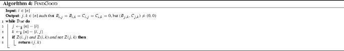
Now we build a function FindGood(i) (Algorithm 4), whose purpose is, given i, to find (j, k) such that $B_{i,j} = B_{i,k} = C_{i,j} = C_{i,k} = 0$, but $(B_{j,k},C_{j,k}) \not = (0,0)$. Why this is useful will become apparent in the next algorithm. To achieve its goal, FindGood picks j, k randomly until Z(i, j) and Z(i, k) hold, but not Z(j, k). This is the case with probability roughly $2^{-6}$, and there are $n(n-1)/2$ choices for j, k so the probability of failure is negligible. Now we explain the point of FindGood.

Let $(\lambda ,\mu ) = (B_{j,k},C_{j,k})$. The point of having the conditions at the output of FindGood is that due to Eq.6, they imply:

$$\begin{aligned} \forall l, ~~ P_{i,j,k,l} = \lambda B_{i,l} + \mu C_{i,l}, \end{aligned}$$

so we recover $(\lambda B + \mu C)_{i,l}$ for all l simply by looking at $P_{i,j,k,l}$. For simplicity we assume $(\lambda ,\mu ) = (1,0)$, and so we are recovering $B_{i,l}$ (other cases correspond to the other two nonzero elements of $\mathrm{span}\{B,C\}$, which as pointed earlier cannot be distinguished from B). If we view B as an $n \times n$ symmetric binary matrix with entries $B_{i,j}$, this means we recover a row of B, namely $B_{i,*}$. This is precisely what we do in algorithm GetSpace(i) (Algorithm 5), which recovers $\mathrm{span}\{B_{i,*},C_{i,*}\}$.

For all i we now know $\mathrm{span}\{B_{i,*},C_{i,*}\}$. All that remains to do in order to build B (or C, or $B+C$) is to choose a nonzero element of GetSpace(0) as the first row; then an element of GetSpace(1) as the second row; and so forth. At each step i, we make sure that our choice of elements is coherent up to this point by checking that the submatrix of rows 0 to i and columns 0 to i is symmetric. If not, we change our choice of element, backtracking if necessary. We name this algorithm Solve (Algorithm 6).

In the end, $\mathrm{span}\{B,C\}$ is recovered as Solve(0, 0, 0) (where the first two parameters are the zero matrix of $\mathbb {F}_{2}^{n \times n}$). Notice that every recursive call to Solve repeats its inner loop twice in case of failure. This is to account for the very rare case where the output of GetSpace might be wrong. Because this case is exceedingly rare, experiments show that repeating the inner loop twice is enough to eliminate such failures. Indeed, our implementation has never returned FAIL on any experiment. On a standard desktop computer this step completes within a second for $n=127$, which is the actual n value for the $\chi$-based $\mathsf {ASASA}$ scheme (see Sect. 1.4 for a link to our implementation).

Application to $\mathsf {ASAS}$ Note that we only need to go through the previous algorithm for the first unperturbed bit in the chain $(z_{0},\dots ,z_{n-p-1})$, namely $z_{0}$. Indeed, we then recover $y'_{0}, y'_{1}, y'_{2}$, and for the next bit we have $z_{1} = y'_{1} + \overline{y'_{2}}y'_{3}$, so only $y'_{3}$ remains to be determined. This can be performed in negligible time, as the system of equations stemming from this equality on the coefficients of $y'_{3}$ is very sparse¹⁰. By induction, we can propagate this process to all other unperturbed bits.

However, in the course of this process we also have to deal with the fact that even from the start, we do not recover $y'_{0}, y'_{1}, y'_{2}$ exactly, but $\mathrm{span}\{y'_{0},y'_{1},y'_{2},1\}$ and $\mathrm{span}\{y'_{1},y'_{2},1\}$. Thus we need to guess $y'_{0}, y'_{1}, y'_{2}$ from the elements of these two vector spaces, then start the process of rebuilding the rest of the chain $(y'_{0},\dots ,y'_{n-p-1})$ as in the previous paragraph. In our experiments, it turns out that as long as $p \ge 2$, there are always exactly 8 solutions for the chain of degree-2 polynomials $(y'_{0},\dots ,y'_{n-p-1})$.

To understand why, we need to look at the last unperturbed bit $z_{n-p-1}$. For this bit, we recover $\mathrm{span}\{y'_{n-p-1},y'_{n-p},y'_{n-p+1},1\}$ and $\mathrm{span}\{y'_{n-p},y'_{n-p+1},1\}$. We can recognize $y'_{n-p-1}$ in the first space (or rather $\mathrm{span}\{y'_{n-p-1},1\}$) because it is also one of the factors in the expression of $z_{n-p-2}$. We can also identify $\mathrm{span}\{y'_{n-p},1\}$ for the same reason. However, there is fundamentally no way to tell $y'_{n-p-1}$ apart from $\overline{y'_{n-p-1}}$, and likewise for $y'_{n-p}$, $y'_{n-p}$, because the necessary information is erased from the public key by the perturbation. For $y'_{n-p}$ for instance, we could flip the $(n-p)$-th bit in the constant $C_{1}$ of $A^{y}$ and also flip the perturbed bit $z_{n-p}$ and this would flip $y'_{n-p}$ without changing $(z_{0},\dots ,z_{n-p-1})$. Thus all 8 solutions for $(y'_{0},\dots ,y'_{n-p-1})$ are valid in the sense that they correspond to equivalent keys, and we are free to choose one of them arbitrarily.

Finally, up to this stage of the attack, we have pretended that $C^{z} = 0$. This actually has no impact on any algorithm so far, except the one just above. With nonzero $C^{z}$, we have $\langle F | a_{i}\rangle = z_{i} + c_{i}$ for $c = (A^{z})^{-1}C^{z}$. This merely adds another degree of freedom in the construction of the previous chain: We guess $c_{0}$ and attempt to go through the process of building the chain. If our guess was incorrect the algorithm fails after two iterations. Once it goes through for two iterations we guess $c_{1}$ and attempt one more iteration, and so forth. Since the chain-building step has negligible complexity, this takes up negligible time.

Overall our algorithm is able to solve Problem 1 for the full $n=127$ within a second on a laptop computer. Thus the time complexity of this step is negligible.

5.4 Peeling off the Remaining $\mathsf {ASA}$ layers

From $\mathsf {ASA}$ to $\mathsf {SA}$ At the end of the previous step we have recovered the chain $(y'_{0},\dots ,y'_{n-p-1})$ of polynomials at the output of $A^{y}$. Now we are left with the task of recovering $A^{x}$, $\lfloor A^{y} \rfloor _{n-p}$ from $H = \lfloor A^{y} \circ \chi \circ A^{x} \rfloor _{n-p}$. Up to now we have always taken advantage of the very simple action of $\chi$ when considering only a single output bit. However, because $A^{y}$ is truncated, we cannot expect that there exist linear masks on the truncated output of $A^{y}$ that give us access to a single bit at the output of $\chi$. For this reason, we switch gear and set out to remove the first layer $A^{x}$ instead.

First, we want to compute the linear component $L^{x}$ of $A^{x}$. Let $\varDelta = \{(L^{x})^{-1} e_{i} : i < n\}$ denote the set of differences $\delta$ that activate only a single bit at the input of $\chi$. Observe that a single bit difference at the input of $\chi$ only affects 3 output bits. As a result, we have an oracle $\mathcal {O}$ that recognizes elements of $\varDelta$: Namely for $\delta \in \varDelta$, the output of $H' = \partial H/\partial \delta$ has dimension only 3 as x spans $\{0,1\}^{n}$.

Furthermore, a closer look reveals that if we remove the constant component in the output of $H'$, then the output of $H'$ has dimension only 2. The reason for this is that, while each bit at the input of $\chi$ affects 3 bits at the output, only 2 bits are affected in a nonlinear manner; and since we are differentiating H, the linear component of $\chi$ only affects the constant component in the output of $H'$.

Let us define an input difference $\delta$ as a vector of n binary unknowns. Then we can formally compute the function $H'$. Assume $\delta \in \varDelta$. Per the previous observation, we know that the linear component of $H'(x)$ has dimension only two as x spans $\{0,1\}^{n}$. That is, for any pairwise distinct $k_{0}, k_{1}, k_{2} < n-p$, there exists a nonzero vector $(\lambda _{0}, \lambda _{1}, \lambda _{2})$ such that $\sum \lambda _{i}H'_{k_{i}} = C(\delta )$ is constant¹¹.

Now observe that $H'$ has degree only one in its input variables $x_{i}$, and the coefficient of each $x_{i}$ is a linear combination of $\delta _{i}$’s; hence, the above equality gives us n linear conditions on $\delta$. Since $\delta$ lives in a space of dimension n, we can hope that this is enough to recover $\delta$, at the cost of guessing the $\lambda _{i}$’s (only 8 possibilities).

In short, the algorithm so far sums up to:

• 1. Pick pairwise distinct $k_{0}, k_{1}, k_{2} < n-p$ arbitrarily.

• 2. Guess $\lambda = (\lambda _{0}, \lambda _{1}, \lambda _{2})$.

• 3. Write the polynomial equality $\sum \lambda _{i}H'_{k_{i}} = 0$. By looking at the coefficient of each $x_{i}$ in this equality, we have n linear conditions on $\delta$.

Let $K(k,\lambda )$ denote the linear subspace of vectors satisfying these conditions. Then, we know that for every $\delta \in \varDelta$, and every choice of k, there exists $\lambda$ such that $\delta \in K(k,\lambda )$.

Note that the cardinality of $\varDelta$ is $128 = 2^{7}$, while $\lambda$ only contains 3 bits of information. Hence, in order to single out each element of $\varDelta$, we repeat the previous algorithm 3 times. This gives us 3 sets of 8 spaces $K(k,\lambda )$. For every choice of K in each set, we compute the intersection of the spaces ($8^{3} = 2^{9}$ possibilities). This yields $2^{9}$ intersections. By construction, we know that each element of $\varDelta$ is in one of the intersections. So we recover $\varDelta$ by testing every element in every intersection against the oracle $\mathcal {O}$.

There are $2^{9}$ intersections, so the only remaining question is whether some of the intersections have dimension greater than 0 or 1 (which may considerably slow down the algorithm). Our experiments show that this is in fact the case, but the resulting spaces still have very low dimension. This is due to “false positives” caused by differences $\delta$ that activate 2 or 3 differences at the input of $\delta$, but these are quickly weeded out by testing against the oracles $\mathcal {O}$.

We have now recovered the linear component of $A^{x}$. Thus we have access to $\lfloor A^{y} \circ \chi \circ (\oplus C^{x}) \rfloor _{n-p}$, where $\oplus C^{x}$ denotes the addition of the constant $C^{x}$. In order to recover $C^{x}$, we can use the fact that $\chi (v)+\chi (v+e_{i})=e_{i}$ (where $e_{i}$ is the canonical basis of $\mathbb {F}_{2}^{n}$) if and only if $v_{i-1}=v_{i+1}=0$. So for each i, we can flip the bits at position $i-1$ and $i+1$ at the input of $\lfloor A^{y} \circ \chi \circ (\oplus C^{x}) \rfloor _{n-p}$ until the previous equality holds. This allows us to recover $C^{x}$ very quickly.

Overall the complexity of this step can be approximated by $2^{9}$ intersections of 3 spaces of dimension 128, which costs around $2^{9}\cdot 2\cdot (2^{7})^{3} = 2^{31}$, so this step is negligible compared to step 1. In fact, we have implemented this step on the full version of the scheme, and it takes only about a minute to complete on a laptop computer.

From $\mathsf {SA}$ to $\mathsf {A}$ We know $\lfloor A^{y} \circ \chi \rfloor _{n-p}$, and we want to recover $\lfloor A^{y} \rfloor _{n-p}$. Observe that $\chi (0)=0$, so $\lfloor C^{y} \rfloor _{n-p} = F(0)$. Moreover $\chi (e_{i})=e_{i}$ so $\lfloor L^{y}(e_{i}) \rfloor _{n-p} = \lfloor A^{y} \circ \chi \rfloor _{n-p}(e_{i})$ and we are done.

6 A Practical Attack on White-Box $\mathsf {ASASA}$

In this section, we show that the actual security of small-block $\mathsf {ASASA}$ ciphers is much lower than was estimated by Biryukov et al.. We describe a procedure to recover the secret components of such schemes, thus breaking their weak white-box security (Definition 2). Our algorithm relies rather heavily on heuristics, and evaluating its efficiency requires actual implementation. We focused on the smallest white-box instance, 16-bit $\mathsf {ASASA} _{16}$, whose claimed security level is 64 bits. Our algorithm was able to recover its secret components under one minute on a laptop computer.

6.1 Attack Overview

Our general black-box attack from Sect. 4 does not apply, because the block size is too small to allow computing cubes of dimension 50. On the other hand, the small-block size makes it possible to compute the distribution of output differences for a single input difference in very reasonable time. In fact, one can compute and store the entire difference distribution table (DDT) of a 16-bit cipher using just a standard PC. For slightly bigger instances such as a 24-bit cipher, computing and storing the entire DDT is still barely possible, even though it would require 3 TB of space and $2^{48}$ invocations of the cipher; computing the distribution of only a few differences on the other hand remains manageable.

Remark 2

Our attack makes use of the full codebook of the ciphers, which in general may be seen as a very strong requirement. This is, however, only natural in the case of attacking white-box implementations, as the user is actually required to be given the full codebook of the super S-boxes as part of the implementation.

Similarly to the attack of the black-box scheme, it is already enough to recover only one of the external affine (or linear) layers in order to break the security of $\mathsf {ASASA}$. Indeed, this allows to reduce the cipher to either of $\mathsf {ASAS}$ or $\mathsf {SASA}$, which can then be attacked in practical time [12]. Thus we focus on removing the first linear layer. In accordance with the opening remarks of Sect. 4.1, this amounts to finding the image space of each S-box through $(A^{x})^{-1}$.

The general idea of the attack is to create an oracle able to recognize whether an input difference $\delta$ activates one or two S-boxes in the first S-box layer $S^{x}$. More accurately, we create a ranking function $\mathcal {F}$ such that $\mathcal {F}(\delta )$ is expected to be significantly higher if $\delta$ activates only one S-box rather than two.

We present two choices for $\mathcal {F}$ which are both heuristic but nonetheless quite efficient as shown by experiments. Both begin by computing the entire output difference distribution $D(\delta )$ for the input difference $\delta$, i.e. the row corresponding to $\delta$ in the DDT. Then, the value of $\mathcal {F}(\delta )$ is computed from $D(\delta )$.

Walsh transform The idea behind this version of the attack is quite intuitive. If $\delta$ activates only one S-box, then after the first $\mathsf {SA}$ layers, two inner states computed from any two plaintexts with input difference $\delta$ are equal on the output of the inactive S-box. Hence, after the first $\mathsf {ASA}$ layers, they are equal along $2^{8}-1$ nonzero linear masks. Since these masks only traverse a single S-box layer before the output of the cipher, linear cryptanalysis [31] tells us that we can expect some linear masks to be biased at the output of the cipher. On the other hand, if both S-boxes are active in the first round, no such phenomenon occurs, and linear biases on the output differences are expected to be weaker.

In order to measure this difference, we propose to compute, for every output mask a, the value $f(a) = (\sum _{x \in \{0,1\}^{16}}\langle \partial F \partial \delta (x) | a\rangle )-2^{15}$ (where the sum is computed in $\mathbb {Z}$). That is, $2^{-15}f(a)$ is the bias of the output differences $D(\delta )$ along mask a. The function f can be computed efficiently, since it is precisely the Walsh transform of the characteristic function of $D(\delta )$, and we can use a fast Fourier transform algorithm. Then as a ranking function $\mathcal {F}$ we simply choose $\max (f)$, i.e. the highest bias among all output masks¹².

Number of collisions It turns out that performing the Walsh transform is not truly necessary. Indeed, the number of collisions in $D(\delta )$ is higher when $\delta$ activates only 1 S-box; where by number of collisions we mean $2^{15}$ minus the number of distinct values in $D(\delta )$. This may be understood as a consequence of the fact that whenever $\delta$ activates a single S-box, only $2^{7}$ output differences are possible after the first $\mathsf {ASA}$ layers; and depending on the properties of the active (random) S-box, the distribution between these differences may be quite uneven. Whereas if both S-boxes are active, $2^{15}$ differences are possible and the distribution is expected to be less skewed. Thus we pick as ranking function $\mathcal {F}$ the number of collisions in $D(\delta )$ in the previous sense.

Once we have chosen a ranking function $\mathcal {F}$, we simply compute the ranking of every possible input difference, sort the differences, and choose the highest 16 linearly independent differences according to our ranking. Our hope is that these differences only activate a single S-box. In a second step, we will group together differences that activate the same S-box.

6.2 Attack Description

We now describe the attack in detail. We focus on the collision ranking function, which is slightly more efficient in practice.

First step We wish to recover the individual components of the $\mathsf {ASASA} _{16}$ cipher ${ A }^z \circ { S }^y \circ { A }^y \circ { S }^x \circ A^x$. The first step of our attack consists in finding 16 linearly independent input differences to the cipher such that only one of the two S-boxes of ${ S }^x$ is active. In other words, we want to find a family of differences $\delta _i$ such that for all i, ${ A }^x(\delta _i)$ is zero in its 8 most significant or 8 least significant bits. As ${ A }^x$ is invertible, there are $2 \times (2^8 - 1)$ nontrivial such differences, but we need an efficient way to test if a given difference is one of them. This can be done by considering the distribution of its corresponding output differences, and counting the number of collisions, as outlined in the previous section.

That is, we attempt to recover 16 suitable differences $\delta _i$ by computing the entire DDT of $\mathsf {ASASA} _{16}$, sorting the input differences by their decreasing number of collisions, and selecting the first 16 linearly independent entries. We describe this formally as Algorithm 7.

Complexity analysis (Algorithm 7). Computing one iteration of Line 2 requires $2^{16}$ calls to $\mathsf {ASASA} _{16}$, each one corresponding to one memory access, and at most $2^{16}$ words of temporary storage. The loop of Line 1 therefore requires $2^{32}$ calls in total and $2^{17}$ words of memory, including $\mathcal {F}$. The sorting of Line 3 can be done in about $2^{20}$ accesses to $\mathcal {F}$ and does not require additional memory. The loop of Line 6 has negligible cost. The total time complexity is thus of the order of $2^{32}$ memory accesses and the memory complexity of the order of $2^{17}$ words (about $2^{18}$ bytes in this case), which are, respectively, quadratic and linear in the size of the domain of $\mathsf {ASASA} _{16}$.

Second step From the previous step, we know 16 input differences $\mathbb {D}[i]$ that each activate only one S-box of ${ S }^x$, and we can now use this knowledge to recover the first layer ${ A }^x$. Similarly to the attack of the black-box scheme of Sect. 4, it is not possible to uniquely determine ${ A }^x$, but it is enough to recover one of the equivalent mappings and later choose the affine equivalent representation of the S-boxes accordingly. The consequence of this is that we only need to identify two groups of 8 linearly independent $\mathbb {D}[i]$’s, respectively, activating the first and the second S-box. Once this is done, we may assume any value for the images of a group as long as they are linearly independent and indeed activate only one S-box.

In order to achieve our goal, we can use the fact that sums of differences of a single group still activate only one S-box, while if the differences come from two groups they obviously activate two. We can use the same method as in the first step to determine whether a sum activates one or two S-boxes, and thence we may hope to find the correct grouping by ensuring that every linear combination of a group (or equivalently every combination of two differences of a group) only activates a single S-box.

We can conveniently describe the resulting problem with a weighted graph and solve it with a simple greedy algorithm. We define the vertices of the graph as being the differences $\mathbb {D}[i]$, and draw an edge between every pair (thus making the graph complete); the weight of the edge $(\mathbb {D}[i], \mathbb {D}[j])$ is defined as the ranking $\mathcal {F}(\mathbb {D}[i]+\mathbb {D}[j])$ of $\mathbb {D}[i]+\mathbb {D}[j]$. The two partitions of 8 differences are then initialized arbitrarily, with their weight defined as the sum of the weight of edges between vertices belonging to the same partition. Finally, the following process is iterated until a fixed point is reached: For any pair of vertices in different partitions, the pair is swapped if and only if this would result in increasing the weight of the partition. We describe this formally as Algorithm 8.

Complexity analysis (Algorithm 8). Assuming that the computations of Line 4 have been cached when running Algorithm 7, every individual step can be computed with negligible time and memory. We then only need to estimate how many times the loop of Line 7 is executed before exiting on Line 16. First it is easy to see that the algorithm does indeed eventually terminate, as ${{\mathrm{\mathcal {W}}}}(\mathbb {S}_1) + {{\mathrm{\mathcal {W}}}}(\mathbb {S}_2)$ increases every time there is as swap of differences. Then, because there are at most $\left( {\begin{array}{c}16\\ 8\end{array}}\right) = 12870$ partitions to consider, we know that the process stops within this number of iterations. In practice, it is unlikely for two S-boxes to be swapped more than once, and the observed time complexity is actually very small.

6.3 Experimental Results and Discussion

We implemented the previous algorithm in C++. The implementation was able to recover the first linear layer of 16-bit $\mathsf {ASASA}$ in a minute on average. This strongly invalidates the security level of 64 bits estimated by [2].

Moreover we implemented a faster but more heuristic algorithm in the Sage formal computation language [39]. This variant uses an oracle $\mathcal {O}$ that predicts whether a difference $\delta$ activates one or two S-boxes, rather than a ranking function. The oracle simply calls the ranking function, and decides that $\delta$ activates a single S-box if $\mathcal {F}(\delta )$ is above a certain threshold. The threshold is determined by comparing values of $\mathcal {F}$ for $\delta$’s that activate one S-box, versus values obtained when $\delta$ activates both S-boxes (this computation only occurs once, by picking a known but random instance and performing the measure).

The algorithm then proceeds by picking random $\delta$’s and using the oracle to check whether $\delta$ activates a single S-box. Once 16 such linearly independent $\delta$’s are found the first step is complete. The second step is identical to the original algorithm. Each $\delta$ has probability $2^{-8}$ of activating a single S-box. Hence, the expected number of $\delta$’s that will need to be tested is $16\cdot 2^{8} = 2^{24}$, which is lower than the $2^{32}$ DDT row computations incurred by the original algorithm. However, this algorithm requires the existence of a clean threshold between the two cases for $\delta$’s.

Sage is a high-level interpreted language, which makes it significantly slower than an equivalent implementation in C++. Nonetheless due to its lower complexity, the previous algorithm was also able to succeed in a minute on average, with either choice of the ranking function $\mathcal {F}$.

All of the implementations are publicly available on the Internet with a link provided in Sect. 1.4.

Remark 3

An interesting observation is that both ranking functions distinguish $\delta$’s that activate one or two S-boxes much less efficiently if $A^{y}$ is maximum distance separable (MDS). However, the attack still goes through, meaning that relying on such matrices is not a suitable countermeasure.

6.4 Adapting the Algorithm to Larger White-Box Instances

The algorithm from the previous section can be adapted to larger white-box instances in a straightforward manner. However, the required computational power is higher. Beside the 16-bit instance, we have also successfully run the attack on the 20-bit instance.

7 Conclusion

We presented a new algebraic attack able to efficiently break both the $\chi$-based public-key cryptosystem and the secret-key scheme of [2]. In addition we proposed another attack that heuristically reduces the key-recovery problem on the $\chi$ scheme to an easy instance of $\mathsf {LPN}$. In the case of the public-key scheme, both attacks go through regardless of the amount of perturbation. For both schemes, the attacks are quite structural (in the case of the black-box scheme, it is in fact structural in the sense of [12]), and seem difficult to patch. Finally, although the general attack on the black-box scheme does not carry over to the small-block instances used for white-box designs, we also showed a very efficient dedicated attack on some of the small-block instances, casting a doubt on their general suitability for that purpose.

Appendices

Omitted Proofs

1.1 Lower Bounding the Number of Linear Relations in Sect. 4.2, step 2

The problem may be formalized as follows. We are given $\alpha , \beta \in \mathbb {F}_{2}^{r}$. The set of $\mu \in \mathbb {F}_{2}^{r}$ such that $\sum \mu _{i}(\alpha _{i},\beta _{i}) = (0,0)$ is (isomorphic to) the annihilator A of $\mathrm{span}\{\alpha ,\beta \}$ in the dual space $(\mathbb {F}_{2}^r)^{*}$. Let $M = \mathbb {F}_{2}^{n \times n}$ denote the space of $n\times n$ binary matrices, with basis $e_{i,j}$. Let $D = \mathrm{span}(\{e_{i,i}^{*}\}\cup \{e_{i,j}^{*}+e_{j,i}^{*}\})$. The space D is isomorphic to the annihilator of $E = \mathbb {F}_{2}^{n(n-1)/2}$; that is, the space of the $\lambda _{i,j}$’s in Sect. 4.2. Let $B = \mathrm{span}\{\sum \mu _{i}e_{i,j}^{*}: \mu \in A, j > r\}$.

The point of the previous definitions is that the linear relations on E obtained from Eq. 1 for $j>r$ are exactly the vectors of the space $B \cap D$.

First, we prove that $\dim B \ge (r-2)(n-r)$. Clearly the projection of B on $C_{j} = \mathrm{span}\{e_{i,j}^{*}:i<n\}$ (which may be seen as looking at a column in the space M) has dimension $\dim A$ for $j > r$. Since $\sum C_{j} \subseteq B$ and the $C_{j}$’s are disjoint, we have $\dim B \ge (n-r)\dim A \ge (r-2)(n-r)$ since A is the annihilator of a space of dimension 2.

Now it remains to show that $\dim (B \cap D) = \dim B$. To see this, it suffices to observe that every functional $e_{i,i}^{*}$ and $e_{i,j}^{*}+e_{j,i}^{*}$ involves a distinct basis element $e_{i,j}^{*}$ for which $i\le j$, whereas B is entirely disjoint from the span of those elements.

1.2 Inversion Algorithm for $\lambda$

Recall that $\lambda : \mathbb {F}_{2}^{n}\times \mathbb {F}_{2}^{n} \rightarrow E$ is defined by $\lambda (a,b)_{i,j} = a_{i}b_{j}+a_{j}b_{i}$. We note that $\lambda$ is symmetric bilinear and $\forall a, \lambda (a,a) = 0$. As a consequence $\lambda (a,b) = \lambda (a+b,b) = \lambda (a,a+b)$. Moreover $\lambda (a,b) = 0$ if and only if a, b are linearly related; indeed, the image of $\lambda (a,b)$ is the set of all determinants of $2 \times 2$ submatrices of the $2 \times n$ matrix whose rows are a and b, i.e. the set of all 2-minors of the matrix.

As a consequence of the previous properties, by inverting $\lambda$, we mean recovering one of $\{a,b\}, \{a+b,b\}, \{a,a+b\}$ given $\lambda (a,b)$, and provided $\lambda (a,b) \not = 0$ (otherwise any linearly dependent a, b is a preimage). For this purpose we use the following algorithm. Consider the $n \times n$ matrix M such that $M_{i,j} = \lambda (a,b)_{i,j}$. Let $R^{i}$ denote the i-th row of M, i.e. $R^{i}_{j} = a_{i}b_{j} + a_{j}b_{i}$. Then observe that $R^{i} = a_{i}b + b_{i}a$. Thus we see that M has rank 2, and in order to invert $\lambda$ in the previous sense, we need only pick any two linearly independent rows of M.

Regarding the Location of Perturbation Polynomials

For the sake of simplicity, in Sect. 5.1, we assumed that perturbation polynomials are contiguous. In order to increase the security of the scheme one could propose to make the positions of perturbations secret. However, this would fail as the scheme would still be broken in practical time. Indeed, according to our experiments, knowing 10 outputs of $\mathsf {ASA}$ among the 127 is enough to perform step 5 and quickly recover the first affine layer $A^{x}$ with a probability of 97% (100 trials with $n = 127$). Thus, as long as there are less than 60 perturbations, one can perform the whole attack to retrieve the first affine layer. Then, in order to retrieve the lines of $(A^{z})^{-1}$ and $A^{y}$ corresponding to unperturbed bits, one need only solve $\text {deg}(P \cdot G) = 4$ where P is an affine combination of the n public polynomials and G is an affine combination of $\chi$. In practice we found this quadratic system to be easily solvable¹³ because of the structure of the scheme. The missing lines can take any value as long as the resulting layers are invertible, each choice determining the perturbation layer.

On the Relationship Between the Problem Encountered in Sect. 5.2 and Learning Parity with Noise

In Sect. 5.2, we encounter a problem related to the Learning Parity with Noise ($\mathsf {LPN}$) problem. In this appendix, we state the problem we encounter more formally and take a closer look at its relationship with $\mathsf {LPN}$. It should be stressed, however, that from a practical perspective, all that matters is that $\mathsf {BKW}$ applies to our problem, and the relationship with $\mathsf {LPN}$ we explore in this appendix is merely of theoretical interest. The main point is that our problem can be properly regarded as a variant of $\mathsf {LPN}$ (rather than a distinct problem to which $\mathsf {BKW}$ happens to also apply).

For convenience, we first recall $\mathsf {LPN}$ as defined in Sect. 2.

Problem 2

($\mathsf {LPN}$) For parameters (n, N, p) with $n < N$ two integers and $p \in (0,1/2)$, an instance of $\mathsf {LPN}$(n, N, p) is defined as follows: given $(A,As + e)$, find s, where:

• $s\in \mathbb {F}_{2}^{n}$ is a uniformly random secret vector.

• $A \in \mathbb {F}_{2}^{N \times n}$ is a uniformly random binary matrix.

• $e \in \mathbb {F}_{2}^{N}$ is an error vector, whose coordinates are chosen according to a Bernoulli distribution with parameter p (i.e., equal to 1 with probability p).

We now model our problem as follows. That is, Problem 3 is essentially the problem we want to solve in Sect. 5.2, disregarding extra structure stemming from the hidden underlying $\mathsf {ASASA}$ structure.

Problem 3

($\mathsf {P}$) For parameters (k, n, N, p) with $k< n < N$ three integers and $p \in (0,1/2)$, an instance of $\mathsf {P}$(n, k, N, p) is defined as follows: given matrix A as below, find $s_1, \dots , s_k$, where:

• $s_1, \dots , s_k \in \mathbb {F}_{2}^{n}$ are secret vectors chosen uniformly at random, conditioned on being linearly independent.

• $e_1, \dots , e_k \in \mathbb {F}_{2}^{N}$ are error vectors, whose coordinates are chosen independently according to a Bernoulli distribution with parameter p.

• $A \in \mathbb {F}_{2}^{N \times n}$ is a matrix whose i-th row is chosen uniformly at random among vectors $v \in \mathbb {F}_2^n$ that satisfy $\langle v | s_j \rangle = e_j(i)$ for all $j \in \{1,\dots ,k\}$.

To relate Problem 3 with the problem from Sect. 5.2, take $n = 127$ to be the number of bits at the input of the $\chi$-based $\mathsf {ASASA}$ instance under attack, $k = n - p = 103$ to be the number of unperturbed bits, and A to be precisely the matrix we build at the beginning of Sect. 5.2. The secret vectors $s_1, \dots , s_n$ are of course the masks we wish to recover, and $p = 1/2 + 2^{-5}$ is the noise rate.

At first sight it may seem that Problem 3 is somewhat different from $\mathsf {LPN}$. However, we show to the contrary that both problems can be reduced to each other. Thus we regard Problem 3 as merely another variant of $\mathsf {LPN}$.

To start, we show that $\mathsf {P}$(1, n, N, p) is essentially the same as $\mathsf {LPN}$ $(n-1,N,p)$. We will tackle the case of $\mathsf {P}$(k, n, N, p) for $k>1$ later; we begin with $k=1$ for simplicity. To make our claim more precise, we say that a problem is $(t,\epsilon )$-solvable if there exists a (probabilistic) algorithm solving it in time t with probability of success $\epsilon$.

Claim

If $\mathsf {P}$(1, n, N, p) is $(t,\epsilon )$-solvable, then $\mathsf {LPN}$ $(n-1,N,p)$ is $(t+\mathcal {O}(n^3),\epsilon )$-solvable. Conversely, if $\mathsf {LPN}$ $(n-1,N,p)$ is $(t,\epsilon )$-solvable, then $\mathsf {P}$(1, n, N, p) is $(t,\epsilon /2)$-solvable.

Proof

Let $\mathcal {A}$ be an algorithm solving $\mathsf {P}$(1, n, N, p) in time t with success probability $\epsilon$. Let (A, b) be an instance of $\mathsf {LPN}$ $(n-1,N,p)$, with $b = As+e$. Define $A'$ to be the $N \times n$ binary matrix obtained by appending column b to matrix A. Similarly, define $s'$ to be the n-dimensional binary vector obtained by appending 1 to s. Pick M a uniformly random invertible $n \times n$ matrix, and let $A'' = A'M$. Then it suffices to observe that $A''$ is an instance of $\mathsf {P}$(1, n, N, p): Its secret vector is $s_1 = M^{-1}s'$ and the error vector is still e. Note that $s_1$ is uniformly random (among nonzero vectors) as required due to the uniform randomness of M. We can then run $\mathcal {A}$ on $A''$ and recover $s' = Ms_1$. Upper-bounding the cost of inverting an $n \times n$ binary matrix by $\mathcal {O}(n^3)$, we obtain the claimed result.

Conversely, let $\mathcal {B}$ be an algorithm solving $\mathsf {LPN}$ $(n-1,N,p)$ in time t with success probability $\epsilon$. Let B be an instance of $\mathsf {P}$(1, n, N, p) with secret vector $s_1$. Now split B into an $N \times (n-1)$ binary matrix $B'$ formed of the first $n-1$ columns of B, and a vector b of dimension N formed of the last column of B. If the last coordinate of $s_1$ is 1, which happens with probability 1 / 2, then $(B',b)$ is an instance of $\mathsf {LPN}$ $(n-1,N,p)$, whose secret vector is the truncation of $s_1$ to its first $n-1$ coordinates. The uniform randomness of the instance directly follows from the uniform randomness of the original one. Hence, we can solve it using $\mathcal {B}$, and recover $s_1$. This proves the claim. The success probability is halved because we had to guess that the last coordinate of $s'_1$ is 1. Note that we could increase this probability by re-randomizing the original instance (i.e., replacing B by BM for a uniformly random invertible M) and reiterating the process (this is essentially due to the random self-reducibility of $\mathsf {LPN}$ and independent of our particular reduction). $\square$

In fact, the previous property can be generalized to $\mathsf {P}$(k, n, N, p) for $k>1$ in a natural way, as shown below. The proof follows the same outline: In order to reduce $\mathsf {LPN}$ to $\mathsf {P}$, we add b to the matrix A and re-randomize (adding also $k-1$ other “artificial” solutions to match an instance of $\mathsf {P}$ with $k>1$). Conversely to reduce $\mathsf {P}$ to $\mathsf {LPN}$ we guess partial solutions, in much the same way that we guessed one bit of the solution in the previous proof. First, we need a simple combinatorial claim.

Claim

If we pick k elements uniformly at random among a set of size $k^2$, then the probability that all elements are pairwise distinct is lower-bounded by 1 / 4.

Proof

The probability that all elements are distinct is:

$$\begin{aligned} \prod _{0 \le i < k} \frac{k^2-i}{k^2} > \left( 1 - \frac{1}{k}\right) ^k \sim e^{-1} \end{aligned}$$

so it is clear that it is lower-bounded by a constant. Moreover basic functional analysis shows that $\left( 1 - \frac{1}{k}\right) ^k$ is increasing, so it can be lower-bounded by $\left( 1 - \frac{1}{2}\right) ^2 = \frac{1}{4}$ for $k \ge 2$. Hence, so can the original probability, and since it is 1 for $k=1$ we get the result. $\square$

Claim

If $\mathsf {P}$(k, n, N, p) is $(t,\epsilon )$-solvable, then $\mathsf {LPN}$ $(n-k,N,p)$ is $(t+\mathcal {O}(n^3),\epsilon )$-solvable. Conversely, if $\mathsf {LPN}$ $(n-\lceil 2\log (k)\rceil ,N,p)$ is $(t,\epsilon )$-solvable, then $\mathsf {P}$(k, n, N, p) is $(2^{\lceil 2\log (k)\rceil }(t + \mathcal {O}(n^3)),\epsilon ^k/4)$-solvable for sufficiently high N.

Proof

Let $\mathcal {A}$ be an algorithm solving $\mathsf {P}$(k, n, N, p) in time t with success probability $\epsilon$. Let (A, b) be an instance of $\mathsf {LPN}$ $(n-k,N,p)$, with $b = As+e$. Let $b_1 = b$, $s_1 = s$ and $e_1 = e$, so $b_1 = As_1+e_1$. We now define $k-1$ “artificial” instances of $\mathsf {LPN}$ $(n-k,N,p)$ with known secrets sharing the same matrix A. That is, pick $s_2, \dots , s_k$ uniformly at random in $\mathbb {F}_2^{n-k}$, $e_2, \dots , e_k$ in $\mathbb {F}_2^{n-k}$ with each coordinate following an independent Bernoulli distribution of parameter p, and define $b_2, \dots , b_k$ by $b_i = As_i + e_i$. Let $s'_i$ denote the n-dimensional vector obtained by appending $f_i$ to $s_i$, where $f_i \in \mathbb {F}_2^{k}$ is the vector satisfying $f_i(i) = 1$ and $f_i(j) = 0$ for $j \ne i$.

Now build the $N \times n$ binary matrix $A'$ obtained by appending $b_1, \dots b_k$ (viewed as column vectors) to A. As in the previous proof, re-randomize the instance by picking a uniformly random invertible $n \times n$ matrix M, and let $A'' = A'M$. Then it suffices to observe that $A''$ is an instance of $\mathsf {P}$(k, n, N, p): Its secret vectors $(s_i)_{i \le k}$ are defined by $s''_i = M^{-1}s'_i$ and the error vector is still e. Note that the $s''_i$’s are uniformly random (conditioned on being linearly independent) by construction due to the uniform randomness of M. We can then run $\mathcal {A}$ on $A''$ and recover $s'_i = Ms''_i$ for all i, in particular we recover $s_1$. Upper-bounding the cost of inverting an $n \times n$ binary matrix by $\mathcal {O}(n^3)$, we obtain the claimed result.

Conversely, let $\mathcal {B}$ be an algorithm solving $\mathsf {LPN}$ $(n-\lceil 2\log (k)\rceil ,N,p)$ in time t with success probability $\epsilon$. Let B be an instance of $\mathsf {P}$(k, n, N, p) with secret vectors $s_1, \dots , s_k$. The general idea is that we simply guess a secret vector on its last $\lceil 2\log (k)\rceil$ coordinates. Moreover, we assume that all vectors $s_1, \dots , s_k$ are pairwise distinct on their last $\lceil 2\log (k)\rceil$ bits, which holds with probability at least 1 / 4 by the previous claim.

Now, for each nonzero vector $s \in \mathbb {F}_2^{\lceil 2\log (k)\rceil }$ (representing a partial guess), we generate an instance of $\mathsf {LPN}$ $(n-\lceil 2\log (k)\rceil ,N,p)$ as follows. Let $B'$ be the $N \times (n-\lceil 2\log (k)\rceil )$ binary matrix obtained by removing the last $\lceil 2\log (k)\rceil$ columns of B. Let $s'$ be the n-dimensional vector obtained by prepending zeros to s, and define $b_s = Bs'$. The crux of the matter is that if s is the truncation of $s_i$ for one single choice of i, then $(B',b_s)$ is a valid instance of $\mathsf {LPN}$ $(n-\lceil 2\log (k)\rceil ,N,p)$. Moreover all instances for various choices of s can be made independent by re-randomizing the instance (i.e., replacing $B'$ by $B'M$ for uniformly random M). On the other hand most choices of s (namely, those that are not a truncation of some $s_i$) will not yield an instance of $\mathsf {LPN}$, but rather a uniformly random matrix. These can be weeded out with high probability by checking that the output of the call to $\mathsf {LPN}$ $(n-\lceil 2\log (k)\rceil ,N,p)$ yields a correct result (which requires N to be high enough that a correct answer can be distinguished from an incorrect one with high probability). In the end we need to run $2^{\lceil 2\log (k)\rceil }$ instances of $\mathsf {LPN}$ $(n-\lceil 2\log (k)\rceil ,N,p)$ to recover all solutions, and pay a price 1 / 4 due to the hypothesis that all k solutions are distinct on their last $\lceil 2\log (k)\rceil$ bits. As in the case $k=1$, however, note that we can increase this probability by re-randomizing the initial instance and reiterating the process. $\square$

Going back to the occurence of Problem 3 in Sect. 5.2, we note that we could in principle use the previous reduction to get an instance of $\mathsf {LPN}$ before applying $\mathsf {BKW}$. However, this would incur an unnecessary loss in the reduction: Indeed, we can heuristically expect that $\mathsf {BKW}$ can be applied directly to the instance of $\mathsf {P}$ as argued in Sect. 5.2.

References

M. R. Albrecht, J. C. Faugère, R. Fitzpatrick, L. Perret, Y. Todo, and K. Xagawa, Practical cryptanalysis of a public-key encryption scheme based on new multivariate quadratic assumptions, in Hugo Krawczyk, editor, Public-Key Cryptography–PKC 2014, Lecture Notes in Computer Science, vol. 8383 (Springer, Berlin, 2014) pp. 446–464
A. Biryukov, C. Bouillaguet, and D. Khovratovich, Cryptographic schemes based on the ASASA structure: black-box, white-box, and public-key, in Palash Sarkar and Tetsu Iwata, editors, Advances in Cryptology–ASIACRYPT 2014, Lecture Notes in Computer Science, vol. 8873 (Springer, Berlin, 2014) pp. 63–84. Full version: http://eprint.iacr.org/2014/474.
C. Boura, A. Canteaut, On the influence of the algebraic degree of \( F^{-1} \) on the algebraic degree of \( G\circ F\), in IEEE Transactions on Information Theory, 59(1):691–702, 2013.
A. Biryukov, C. De Canniere, A. Braeken, and B. Preneel, A toolbox for cryptanalysis: Linear and affine equivalence algorithms, in International Conference on the Theory and Applications of Cryptographic Techniques (EUROCRYPT), (Springer, Berlin, 2003) pp. 33–50
L. Bettale, J. -C. Faugère, and L. Perret, Cryptanalysis of multivariate and odd-characteristic HFE variants, in Public Key Cryptography—PKC 2011, vol. 6571 (Springer, Berlin, 2011) pp. 441–458
A. Bhattacharyya, Polynomial decompositions in polynomial time, in Andreas S. Schulz and Dorothea Wagner, editors, Proceedings Algorithms - ESA 2014 - 22th Annual European Symposium, Wroclaw, Poland, September 8–10, 2014., of Lecture Notes in Computer Science vol. 8737 (Springer, Berlin, 2014), pp. 125–136
G. Blom, L. Holst, and D. Sandell, Problems and snapshots from the world of probability. (Springer, Berlin, 2012)
A. Bhattacharyya, P. Hatami, and M. Tulsiani, Algorithmic regularity for polynomials and applications, in Piotr Indyk, editor, Proceedings of the Twenty-Sixth Annual ACM-SIAM Symposium on Discrete Algorithms, SODA 2015, San Diego, CA, USA, January 4-6, 2015, SIAM, 2015 pp. 1870–1889
E. Biham, Cryptanalysis of patarin’s 2-round public key system with s-boxes (2R), in Bart Preneel, editor, Advances in Cryptology – EUROCRYPT 2000, Lecture Notes in Computer Science, vol. 1807 (Springer, Berlin, 2000) pp. 408–416
A. Biryukov and D. Khovratovich, Decomposition attack on SASASASAS, in Cryptology ePrint Archive, Report 2015/646, 2015. http://eprint.iacr.org/.
A. Blum, A. Kalai, and H. Wasserman, Noise-tolerant learning, the parity problem, and the statistical query model, in Journal of the ACM (JACM), 50(4):506–519, 2003.
A. Biryukov and A. Shamir, Structural cryptanalysis of SASAS, in Birgit Pfitzmann, editor, Advances in Cryptology–EUROCRYPT 2001, Lecture Notes in Computer Science, vol. 2045 (Springer, Berlin, 2001) pp. 395–405
S. Bogos, F. Tramer, and S. Vaudenay, On solving LPN using BKW and variants. Cryptography and Communications, 8(3):331–369, 2016.
J. Daemen, Cipher and hash function design strategies based on linear and differential cryptanalysis. PhD thesis, Katholieke Universiteit Leuven, Leuven, Belgium, 1995.
I. Dinur, O. Dunkelman, T. Kranz, G. Leander, Decomposing the asasa block cipher construction, in Cryptology ePrint Archive, Report 2015/507, 2015. http://eprint.iacr.org/2015/507/.
Y. Ding-Feng, K. Y. Lam, and D. Zong-Duo, Cryptanalysis of “2R” schemes, in Michael Wiener, editor, Advances in Cryptology – CRYPTO’ 99, Lecture Notes in Computer Science, vol. 1666 (Springer, Berlin, 1999) pp. 315–325
V. Dubois, P. Alain Fouque, A. Shamir, and J. Stern, Practical cryptanalysis of SFLASH, in Alfred Menezes, editor, Advances in Cryptology - CRYPTO 2007, Lecture Notes in Computer Science, vol. 4622 (Springer, Berlin, 2007) pp. 1–12
V. Dubois, L. Granboulan, J. Stern, Cryptanalysis of HFE with internal perturbation, in Tatsuaki Okamoto and Xiaoyun Wang, editors, Public Key Cryptography – PKC 2007, Lecture Notes in Computer Science, vol. 4450 (Springer, Berlin, 2007) pp. 249–265
W. Diffie and M. E. Hellman, Multiuser cryptographic techniques, in AFIPS 1976 National Computer Conference, (ACM, 1976) pp. 109–112
J. Ding, A new variant of the matsumoto-imai cryptosystem through perturbation, in Feng Bao, Robert Deng, and Jianying Zhou, editors, Public Key Cryptography – PKC 2004, Lecture Notes in Computer Science, vol. 2947 (Springer, Berlin, 2004) pp. 305–318
I. Dinur and A. Shamir, Cube attacks on tweakable black box polynomials, in Antoine Joux, editor, Advances in Cryptology – EUROCRYPT 2009, Lecture Notes in Computer Science, vol. 5479 (Springer, Berlin, 2009) pp. 278–299
H. Fell and W. Diffie, Analysis of a public key approach based on polynomial substitution, in Hugh C. Williams, editor, Advances in Cryptology – CRYPTO ’85 proceedings, Lecture Notes in Computer Science, vol. 218 (Springer, Berlin, 1986) pp. 340–349
J. -C. Faugère and A. Joux, Algebraic cryptanalysis of hidden field equation (HFE) cryptosystems using Gröbner bases, in Dan Boneh, editor, Advances in Cryptology - CRYPTO 2003, Lecture Notes in Computer Science, vol. 2729 (Springer, Berlin, 2003) pp. 44–60
J. -C. Faugère and L. Perret, Cryptanalysis of 2R- schemes, in Cynthia Dwork, editor, Advances in Cryptology - CRYPTO 2006, Lecture Notes in Computer Science, vol. 4117 (Springer, Berlin, 2006) pp. 357–372
J.-C. Faugère and L. Perret. An Efficient Algorithm for Decomposing Multivariate Polynomials and its Applications to Cryptography. J. Symb. Comput., 44(12):1676–1689, 2009.
J.-C. Faugère and L. Perret, High order derivatives and decomposition of multivariate polynomials, in ISSAC ’09: Proceedings of the 2009 International Symposium on Symbolic and Algebraic Computation, (ACM, 2009) pp. 207–214
J.-C. Faugère, J. von zur Gathen, and L. Perret, Decomposition of generic multivariate polynomials, in ISSAC ’10: Proceedings of the 2010 International Symposium on Symbolic and Algebraic Computation, (ACM, 2010) pp. 131–137. isbn: 0747-7171 (updated version).
H. Gilbert, Jérôme Plût, and J. Treger, Key-recovery attack on the ASASA cryptosystem with expanding S-boxes, in CRYPTO 2015. (Springer, Berlin, 2015)
Y. -J. Huang, F. -H. Liu, and B. -Y. Yang, Public-key cryptography from new multivariate quadratic assumptions, in Marc Fischlin, Johannes A. Buchmann, and Mark Manulis, editors, Proceedings Public Key Cryptography - PKC 2012 - 15th International Conference on Practice and Theory in Public Key Cryptography, Darmstadt, Germany, May 21-23, 2012., volume 7293 of Lecture Notes in Computer Science, (Springer, Berlin, 2012) pp. 190–205
É. Levieil and P. -A. Fouque, An improved LPN algorithm, in Roberto De Prisco and Moti Yung, editors, Security and Cryptography for Networks, Lecture Notes in Computer Science, vol. 4116 (Springer, Berlin, 2006) pp. 348–359
M. Matsui, Linear cryptanalysis method for DES cipher, in Tor Helleseth, editor, Advances in Cryptology – EUROCRYPT ’93, Lecture Notes in Computer Science, vol. 765 (Springer, Berlin, 1994) pp. 386–397
T. Matsumoto and H. Imai, Public quadratic polynomial-tuples for efficient signature-verification and message-encryption, in D. Barstow, W. Brauer, P. Brinch Hansen, D. Gries, D. Luckham, C. Moler, A. Pnueli, G. Seegmüller, J. Stoer, N. Wirth, and Christoph G. Günther, editors, Advances in Cryptology – EUROCRYPT ’88, Lecture Notes in Computer Science, vol. 330 (Springer, Berlin, 1988) pp. 419–453
J. Patarin, Cryptanalysis of the Matsumoto and Imai public key scheme of Eurocrypt’88, in Don Coppersmith, editor, Advances in Cryptology – CRYPTO’ 95, Lecture Notes in Computer Science, vol. 963 (Springer, Berlin, 1995) pp. 248–261
J. Patarin, Hidden Fields Equations (HFE) and Isomorphisms of Polynomials (IP): Two New Families of Asymmetric Algorithms, in Ueli Maurer, editor, Advances in Cryptology – EUROCRYPT ’96, Lecture Notes in Computer Science, vol. 1070 (Springer, Berlin, 1996) pp. 33–48
J. Patarin and L. Goubin, Asymmetric cryptography with S-boxes, in ICICS’97, Lecture Notes in Computer Science, vol. 1334 (Springer, Berlin, 1997) pp. 369–380
J. Patarin, L. Goubin, N. Courtois, Quartz, 128-bit long digital signatures, in CT-RSA Conference. (2001)
O. Regev, On lattices, learning with errors, random linear codes, and cryptography, in STOC’05. (ACM Press, 2005), pp. 84–93
V. Rijmen, B. Preneel, A family of trapdoor ciphers, in Eli Biham, editor, Fast Software Encryption, Lecture Notes in Computer Science, vol. 1267 (Springer, Berlin, 1997), pp. 139–148
The Sage Development Team. Sage Mathematics Software. http://www.sagemath.org
H. Wu, F. Bao, R. Deng, Q.-Z. Ye, Cryptanalysis of Rijmen–Preneel Trapdoor Ciphers, in Kazuo Ohta, Dingyi Pei, editors, Advances in Cryptology—ASIACRYPT’98, Lecture Notes in Computer Science, vol. 1514 (Springer, Berlin, 1998), pp. 126–132
Author information
Authors and Affiliations
Corresponding author
Additional information
Communicated by Serge Vaudenay.
Patrick Derbez: Supported by the CORE ACRYPT project from the Fond National de la Recherche, Luxembourg.
Pierre Karpman: Partially supported by the Direction Générale de l’Armement and by the Singapore National Research Foundation Fellowship 2012 (NRF-NRFF2012-06).